


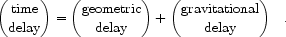
There is a sense in which time delay is the most fundamental manifestation of gravitational lensing. In the weak field limit a gravitational potential produces an effective index of refraction that increases the travel time for a photon. Fermat's principle requires that the photon travel along a path that is a minimum, a maximum or a saddlepoint of the travel time. The photon must detour around the path it otherwise would have taken. A balance is struck between increased travel time associated with the detour (the geometric delay) and decreased travel time due to the shallower gravitational potential (the Shapiro delay),
 |
(3.1) |
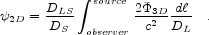
If the size of the lens is small compared to the path length, we can
use the thin lens approximation. The time delay can be expressed in
terms of a two-dimensional effective potential obtained by integrating the
gravitational potential
 3D along the
line of sight,
3D along the
line of sight,
 |
(3.2) |
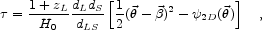
It depends upon the angular diameter distances to the lens and to the source, DL and DS, and upon the distance from the lens to the source, DLS. With this simplification all of gravitational lensing boils down to taking derivatives of the time delay function,
 |
(3.3) |
where
 measures
the position on the sky at which a ray crosses the plane of the lens and
measures
the position on the sky at which a ray crosses the plane of the lens and
 is the position on the
sky of the source. Here we use the dimensionless variants of the
angular diameter distances, dL, dS,
and dLS. The quantity
-
is the amount by which
a ray is deflected. The geometric part of the time delay varies
as the square of deflection in the limit of small deflections,
a straightforward consequence of the Pythagorean theorem.
is the position on the
sky of the source. Here we use the dimensionless variants of the
angular diameter distances, dL, dS,
and dLS. The quantity
-
is the amount by which
a ray is deflected. The geometric part of the time delay varies
as the square of deflection in the limit of small deflections,
a straightforward consequence of the Pythagorean theorem.
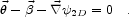
Differentiating  with
respect to
and setting the gradient of
to zero allows us to solve for
the minima, maxima and saddlepoints of the time delay. It gives what is
often call the lens equation,
with
respect to
and setting the gradient of
to zero allows us to solve for
the minima, maxima and saddlepoints of the time delay. It gives what is
often call the lens equation,
 |
(3.4) |
The deflection,
-
,
is equal to the gradient of the two dimensional potential.
The magnification of an image is the ratio of the observed angular
size to the true angular size of an object. We want something
like the ratio of
 to
,
but both of these are vectors. Passing to derivatives, the quantity
to
,
but both of these are vectors. Passing to derivatives, the quantity
 /
gives a magnification matrix that maps a vector at the position of the
source,
,
into a vector in the image plane,
.
This matrix cannot be calculated from equation 4 because the
two dimensional potential is a function of position in the lens plane,
not the source plane. But its inverse can be calculated by taking
the derivative of equation 4 with respect to
,
giving the inverse magnification matrix,
/
gives a magnification matrix that maps a vector at the position of the
source,
,
into a vector in the image plane,
.
This matrix cannot be calculated from equation 4 because the
two dimensional potential is a function of position in the lens plane,
not the source plane. But its inverse can be calculated by taking
the derivative of equation 4 with respect to
,
giving the inverse magnification matrix,
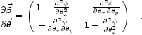 |
(3.5) |
This is readily inverted to give the magnification matrix,
/
.
Since the magnification matrix is
symmetric, there is a choice of coordinates for which it is diagonal.
Those diagonal elements are in general unequal, stretching or
compressing the image more in one direction than the other. The
magnification matrix might equally well be called the distortion matrix.
It is often the case that the source and its images are very much smaller than the resolution of our observations. Gravitational lensing conserves surface brightness, but as the solid angle subtended by the image is usually different from that subtended by the source, the observed flux is also different. The scalar magnification factor, µ, is given by
 |
(3.6) |
The observable consequences of lensing are mnemonized with three "D's," each corresponding to a different derivative of the time delay function. The first derivative of the delay function gives a deflection. The second derivative gives a distortion. And the "zeroth" derivative is just the delay function itself.