6. DESCRIBING DARK ENERGY

The absence of a consensus model for cosmic acceleration presents a challenge in trying to connect theory with observations. For dark energy, the equation-of-state parameter w provides a useful phenomenological description [Turner & White 1997]. Because it is the ratio of pressure to energy density, it is also closely connected to the underlying physics. However, w is not fundamentally a function of redshift, and if cosmic acceleration is due to new gravitational physics, the motivation for a description in terms of w disappears. In this section, we review the variety of formalisms that have been used to describe and constrain dark energy.

6.1. Parametrizations

The simplest parameterization of dark energy is w = const. This form fully describes vacuum energy (w = -1) and, together with _DE and _M, provides a 3-parameter description of the dark-energy sector (2 parameters if flatness is assumed). However, it does not describe scalar field or modified gravity models.

A number of two-parameter descriptions of w have been explored, e.g., w(z) = w₀ + w' z and w(z) = w₀ + bln(1 + z). For low redshift they are all essentially equivalent, but for large z, some lead to unrealistic behavior, e.g., w << -1 or ≫ 1. The parametrization

(22)

(e.g., [Linder 2003]) avoids this problem and leads to the most commonly used description of dark energy, namely (_DE, _M, w₀, w_a)

More general expressions have been proposed, for example, Padé approximants or the transition between two asymptotic values w₀ (at z 0) and w_f (at z ), w(z) = w₀ + (w_f - w₀)/(1+ exp[(z - z_t) / ]) [Corasaniti & Copeland 2003].

The two-parameter descriptions of w(z) that are linear in the parameters entail the existence of a "pivot" redshift z_p at which the measurements of the two parameters are uncorrelated and the error in w_p w(z_p) reaches a minimum [Huterer & Turner 2001]; see the left panel of Fig. 11. The redshift of this sweet spot varies with the cosmological probe and survey specifications; for example, for current SN Ia surveys z_p 0.25. Note that forecast constraints for a particular experiment on w_p are numerically equivalent to constraints one would derive on constant w.

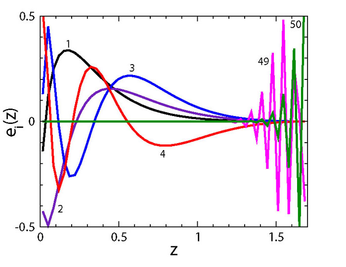Figure 11. Left panel: Example of forecast constraints on w(z), assuming w(z) = w0 + w'z. The "pivot" redshift, zp 0.3, is where w(z) is best determined. From [Huterer & Turner 2001]. Right panel: The four best-determined (labelled 1-4) and two worst-determined (labelled 49, 50) principal components of w(z) for a future SN Ia survey such as SNAP, with several thousand SNe in the redshift range z = 0 to z = 1.7. From [Huterer & Starkman 2003].

6.2. Direct reconstruction

Another approach is to directly invert the redshift-distance relation r(z) measured from SN data to obtain the redshift dependence of w(z) in terms of the first and second derivatives of the comoving distance [Huterer & Turner 1999, Starobinsky 1998],

(23)

Assuming that dark energy is due to a single rolling scalar field, the scalar potential can also be reconstructed,

(24)

Others have suggested reconstructing the dark energy density [Wang & Mukherjee 2004],

(25)

Direct reconstruction is the only approach that is truly model-independent. However, it comes at a price - taking derivatives of noisy data. In practice, one must fit the distance data with a smooth function — e.g., a polynomial, Padé approximant, or spline with tension, and the fitting process introduces systematic biases. While a variety of methods have been pursued (e.g., [Weller & Albrecht 2002, Gerke & Efstathiou 2002]), it appears that direct reconstruction is too challenging and not robust even with SN Ia data of excellent quality. Although the expression for _DE(z) involves only first derivatives of r(z), it contains little information about the nature of dark energy. For a review of dark energy reconstruction and related issues, see [Sahni & Starobinsky 2006].

6.3. Principal components

The cosmological function that we are trying to determine — w(z), _DE(z), or H(z) — can be expanded in terms of principal components, a set of functions that are uncorrelated and orthogonal by construction [Huterer & Starkman 2003]. In this approach, the data determine which components are measured best.

For example, suppose we parametrize w(z) in terms of piecewise constant values w_i (i = 1, . . ., N), each defined over a small redshift range (z_i, z_i + z). In the limit of small z this recovers the shape of an arbitrary dark energy history (in practice, N 20 is sufficient), but the estimates of the w_i from a given dark energy probe will be very noisy for large N. Principal Component Analysis extracts from those noisy estimates the best-measured features of w(z). We find the eigenvectors e_i(z) of the inverse covariance matrix for the parameters w_i and the corresponding eigenvalues _i. The equation-of-state parameter is then expressed as

(26)

where the e_i(z) are the principal components. The coefficients _i, which can be computed via the orthonormality condition, are each determined with an accuracy 1 / (_i)^1/2. Several of these components are shown for a future SN survey in the right panel of Fig. 11.

One can use this approach to design a survey that is most sensitive to the dark energy equation-of-state parameter in some specific redshift interval or to study how many independent parameters are measured well by a combination of cosmological probes. There are a variety of extensions of this method, including measurements of the equation-of-state parameter in redshift intervals [Huterer & Cooray 2005].

6.4. Kinematic description

If the explanation of cosmic acceleration is a modification of GR and not dark energy, then a purely kinematic description through, e.g., the functions a(t), H(z), or q(z) may be the best approach. With the weaker assumption that gravity is described by a metric theory and that spacetime is isotropic and homogeneous, the FRW metric is still valid, as are the kinematic equations for redshift/scale factor, age, r(z), and volume element. The dynamical equations, i.e., the Friedmann equations and the growth of density perturbations, may however be different.

If H(z) is chosen as the kinematic variable, then r(z) and age take their standard forms. On the other hand, to describe acceleration one might wish to take the deceleration parameter q(z) as the fundamental variable; the expansion rate is then given by

(27)

Another possibility is the dimensionless "jerk" parameter, j (a/a)/H³, instead of q(z) [Visser 2004, Rapetti et al. 2007]. The deceleration q(z) can be expressed in terms of j(z),

(28)

and, supplemented by Eq. (27), H(z) may be obtained. Jerk has the virtue that constant j=1 corresponds to a cosmology that transitions from a t^2/3 at early times to a e^Ht at late times. Moreover, for constant jerk, Eq. (28) is easily solved:

(29)

On the other hand, constant jerk does not span cosmology model-space well: the asymptotic values of deceleration are q = q _±, so that only for j = 1 can there be a matter-dominated beginning (q = 1/2). One would test for departures from CDM by searching for variation of j(z) from unity over some redshift interval; in principle, the same information is also encoded in q(z).

The kinematic approach has produced some interesting results; using the SN data and the principal component method, [Shapiro & Turner 2006] find the best measured mode of q(z) can be used to infer 5- evidence for acceleration of the Universe at some recent time, without recourse to GR and the Friedmann equation.