


In the previous section, I outlined the basic theory behind Bondi-Hoyle-Lyttleton accretion. This lead to elegant predictions for the accretion rate, as given by equations 7 and 32. However, reaching these equations required a lot of simplifying assumptions, so necessitating further investigation. The intractability of the equations of fluid dynamics requires a numerical approach to the problem.
In a break with tradition, I shall start this section with the answer, and then give more detailed citations to examples.
Do the equations of Bisnovatyi-Kogan et al. provide a good description of Bondi-Hoyle-Lyttleton flow? The answer is `No.'
In the absence of other effects, three numbers parameterise Bondi-Hoyle-Lyttleton flow:

 HL
HL
 value of the gas
Figure 5 shows sample density
contours for a flow with
= 1.4, an accretor radius of
0.1
HL
and = 5/3.
This particular simulation was axisymmetric.
A bow shock has formed on the upstream side.
The corresponding velocity field is plotted in
figure 6.
Downstream of the shock, material flows almost radially onto the
accretor, in marked contrast to the analytic solution of
equations 8 to 11.
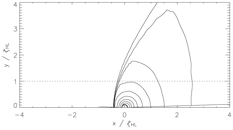 |
Figure 5. Density contours for a sample
Bondi-Hoyle-Lyttleton simulation. The flow had
|
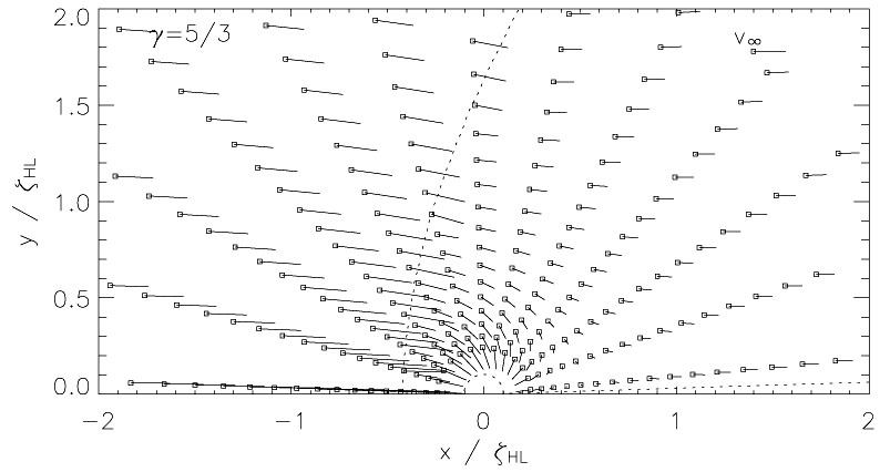 |
Figure 6. Velocity field corresponding to the densities shown in figure 5. The approximate position of the bow shock is marked with a dotted line. |
But what of the accretion rate? Figure 7 shows the accretion rates obtained for three simulations. Although the dimensionless parameters were kept the same, the physical scales and grid resolution varied. Figures 5 and 6 were taken from run 2. The accretion rates achieved are quite close to the value of MHL predicted for the flow (this value is substantially larger than the corresponding MBH). Despite the simplifications made, the work of Bondi, Hoyle and Lyttleton has been largely vindicated. In the remainder of the section, I shall cite places in the literature where further simulations of Bondi-Hoyle-Lyttleton flow may be found.
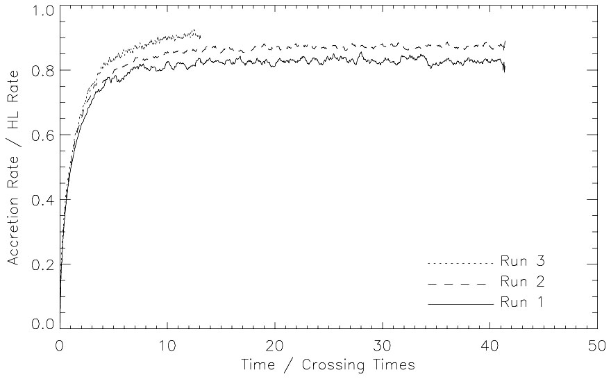 |
Figure 7. Accretion rates for plain
Bondi-Hoyle-Lyttleton flow. The crossing time corresponds to
|
3.2. Examples in the Literature
Hunt computed numerical solutions of Bondi-Hoyle-Lyttleton flow in two papers written in 1971 and 1979. The accretion rate suggested by equation 32 agreed well with that observed, despite the flow pattern being rather different. Hunt studied flows which were not very supersonic and were non-isothermal. A bow shock formed upstream of the accretor. Upstream of the shock, the flow pattern was very close to the original ballistic approximation. Downstream, the gas flowed almost radially towards the point mass. A summary of early calculations of Bondi-Hoyle-Lyttleton flow may be found in Shima et al. (1985). The calculations in this paper are in broad agreement with earlier work, but some differences are noted and attributed to resolution differences.
More recently, a series of calculations in three dimensions have
been performed by Ruffert in a series
of papers
(Ruffert, 1996,
1994a,
1995,
1994b;
Ruffert
and Arnett, 1994).
This series of papers used a code based on nested grids, to permit
high resolution at minimal computational cost.
Ruffert
(1994a)
details the code, and presents simulations
of Bondi accretion (where the accretor is stationary).
Bondi-Hoyle-Lyttleton flow was considered in
Ruffert
and Arnett (1994).
The flow of gas with = 3
and =
5/3 past an accretor of varying sizes (0.01 < r /
BH
< 10) was studied. For accretors substantially smaller than
BH,
the accretion rates
obtained were in broad agreement with theoretical predictions.
The flow was found to have quiescent and active phases, with smaller
accretors giving larger fluctuations.
However, these fluctuations were far less violent than the `flip-flop'
instability observed in 2D simulations (see below).
Ruffert
(1994b)
extended these simulations to cover a range
of Mach numbers, finding that higher Mach numbers tended to give lower
accretion rates (down to the original interpolation formula of
equation 31). Ruffert studied the flow of a gas with
= 4/3
in the 199 paper, finding accretion
rates comparable with the theoretical results.
Small accretors and fast flows were required before any instabilities
appeared in the flow. Nearly isothermal flow was considered in
Ruffert
(1996).
The accretion rates were slightly higher than the theoretical values (except
for the smaller accretors), and the shock moved back to become a tail
shock. The oscillations in the flow were less violent still.
The reason for the formation of the bow shock is straightforward - the
rising pressure in the flow. As shown by equation 11, the flow is
compressed as it approaches the accretor. This compression will increase
the internal pressure of the flow, eventually causing a significant
disruption. At this point, the shock will form. This interpretation is
consistent with the behaviour observed in simulations, where decreasing
moves
the shock back towards the accretor.
However, the precise location of the shock does not seem to be a
strong function of the Mach number (cf the papers of Ruffert).