4. METHODS AND VALIDATION OF SED FITTING

In Section 2 we have described how models predict the SEDs of galaxies. Yet the ultimate goal of these models is to allow the reverse process, that is to derive the properties of galaxies from their observed SEDs through fitting procedures. Therefore we describe in this section several of the main methods used to fit model or observed template SEDs to multiwavelength observations of galaxies. Exactly which of these procedures should be used is contingent on which physical parameters are required and with what precision. In turn, this, and the accuracy with which the models reproduce specific observations, determines what observational data are necessary.

The following sections deal almost exclusively with stellar emission. This reflects a real dearth of specialized codes for carrying out the fitting process in the dust emission range (besides simple ² minimization over a parameter grid, e.g. Klaas et al. 2001). This state of affair is understandable, however, in light of the rapid development and large uncertainties still inherent to our modelling of the dust emission of galaxies.

4.1. Parametrizing SED models

In the context of a SED model, one must distinguish between independent, input parameters and derived parameters. Input parameters are those properties that are needed to define the SED model. Some of them may, first, not be measurable or, second, may not have a proper physical meaning by themselves. A good example for the first case is the shown in Figures 10 and 11 of da Cunha et al. (2008), where the width of the probability distribution functions of different input parameters indicates which ones are well constrained, such as the global contribution of PAHs to the total luminosity, and which are not constrained, such as the temperature of warm dust in stellar birth clouds. Iglesias-Páramo et al. (2007 their Section 3) state another example, namely that only a few of the many input parameters of the GRASIL code need to be varied in order to produce a library of model spectra that cover a realistic range in observational properties. Further, more systematic study of the relative importance of the input parameters to dust emission models would seem to be a important addition to the literature. A good example of the second case is the "decay timescale", _*: in modelling the SEDs of early- and even late-type galaxies, the star formation histories (SFHs) are often represented as falling exponential functions modulated by this timescale, i.e. SFR(t) e^{(-t / _*)}. However, in a hierarchical universe the SFH is likely to be more stochastic in form, modulated by discrete accretion events. Thus the width of the falling exponential that one determines from an SED fit is a good measure of the mean age of the galaxy. It should by no means be assumed that this represents the true SFH of the galaxy. The reason that falling exponentials provide reasonable fits in practice is simply that the spectral features of SSPs vary smoothly with time and there is thus considerable degeneracy between the mass contributions of SSPs of different age, effectively smoothing the SFHs of galaxies. This smoothing makes it also impossible in practice to robustly disentangle the epoch of the formation of the most luminous stellar population in a galaxy from the timescale over which this star formation took place.

Input parameters constitute a discrete set with a maximum number of members determined by the quality of the data and the models. On the other hand the set of derived parameters can be extended at will and not all derived parameters can or need to be independent. For example, the commonly used specific star formation rate (sSFR = SFR / M_*) and the birthrate parameter (b = SFR / < SFR >_t) are derived parameters that are very similar. It is clearly relevant to properly define and understand the derived physical properties that one intends to measure. Let us again consider the SFR. While the SFR derived from the UV flux traces an average SFR over the last 100 Myr, the SFR determined from Balmer emission lines measures the much shorter timescale of the ionizing stellar flux, 10 Myr. These two measures, while correlated, thus need to be properly corrected before being able to compare them (see e.g. Kennicutt 1998, Boquien et al. 2007, Kennicutt et al. 2009, Lee et al. 2009a and references therein).

As an integrated model of the optical SED of a galaxy is based more or less explicitly on an equation similar to Equation 1, the independent and derived parameters should be defined in the same terms (see e.g. Walcher et al. 2008, Table 1). Actually writing down the definition helps avoid common confusions (such as those between metallicity Z and [Fe/H], or concerning the time scale over which the SFR is measured) and should be considered good practice.

4.2. Spectral indices

It has been said in the introduction that SED fitting can only yield useful results if the models are as or more precise than the effect on the data of the property to be measured. Historically this was the case only for very limited wavelength ranges in the optical. The solution to this problem has then been to not fit the entire SED, but to define indices, i.e. measure the equivalent widths, for certain absorption features.

In the standard side-band method (Burstein et al. 1984, Faber et al. 1985) a careful analysis leads to the definition of one central and two side bands (a blue and a red). The continuum compared to which the equivalent width is measured is a linear interpolation between the average fluxes found in these two sidebands. Much work has gone into optimizing the set of available indices, as well in terms of coverage, as well as in terms of model precision (e.g. Rose 1984, Worthey et al. 1994, Trager et al. 1998, Tripicco and Bell 1995, Cenarro et al. 2002, Thomas et al. 2004, Lee et al. 2009b and references therein).

We are still waiting for standard indices in other wavelengths than the optical, though see Rix et al. (2004), Keel (2006), Maraston et al. (2009), & Chavez et al. (2009), and Lançon et al. (2008) & Cesetti et al. (2009) for headway into the UV and NIR respectively. These would make the index approach a true multi-wavelength approach.

Rogers et al. (2010a) have attempted to improve on the classical sideband definition by introducing a "boosted median" method. The main feature of this method is that for each side-band only the Lth percentile of the distribution of fluxes is used to determine the flux within the side-band. As this procedure automatically chooses the largest fluxes in the side-band, it will define the pseudo-continuum from those points that are least affected by "secondary" absorption features, i.e. absorption features that are not part of the central band. It thus improves the robustness of the pseudo-continuum if the spectral resolution is high enough to avoid blending of all features. Figure 9 illustrates the difference between the boosted median equivalent width and a standard side-band method for a measurement of H. The sample corresponds to a set of 14 elliptical galaxies in the Virgo cluster observed with a 2-2.4Å resolution (FWHM) and with high S/N (Yamada et al. 2006).

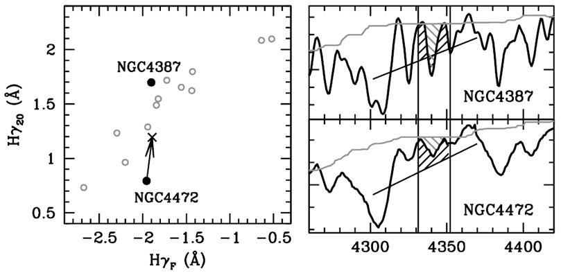Figure 9. Comparison of the HF equivalent width measured with the side-band (SB) and the proposed Boosted Median method (H20; BMC). The black dots mark two galaxies with a significant difference between both methods. On the right-hand panels, the SED of these two galaxies is shown, with the slanted line representing the continuum defined by the SB method, and the gray line showing the BMC pseudo-continuum. The hatched black (gray) regions correspond to the equivalent width according to the side-band (BMC) method. The arrow and cross in the left panel shows the change in equivalent width caused by the difference in velocity dispersion between NGC 4387 (112 km/s) and NGC 4472 (303 km/s). [Courtesy I. Ferreras]

Index fitting can be considered a special case of SED fitting (for a fitting code see e.g. Graves and Schiavon 2008). It has the advantage of compressing the information available in galaxy spectra into a set of discrete numbers. Much of what is considered secure knowledge in stellar element abundances and age of integrated stellar populations is still largely based on fitting indices (e.g. Trager et al. 2000, Kauffmann et al. 2003a, Thomas et al. 2005, Gallazzi et al. 2008, Graves et al. 2009 to cite only a few).

The clear disadvantage of absorption line indices is that some of the information is lost. While indices have been defined with great care to approach the ideal of representing one element species, in practice many small lines interfere in particular in the side-bands. Spectral fitting (Section 4.4) can in principle use more information but it places much higher requirements on model accuracy.

4.3. Principal Component Analysis

Ideally we would like to represent a galaxy spectrum by a small set of continuous parameters that uniquely determine the best-fit spectrum. Principal Component Analysis (PCA) is one algorithm commonly used to derive an optimal set of linear components, diagonalising the covariance matrix of the data points to find the directions of greatest variation. Its representation of data through a linear combination of independent (orthogonal) components, or eigenvectors is thus an alternative method to using a set of discrete SSP templates (Section 4.4). Since the convolution with transmission curves is a linear operation, these methods are as simple as solving a linear equation, even for photometric datasets (Connolly et al. 1999, Budavári et al. 2000).

PCA has been successfully applied to astronomical spectral datasets, although not yet to photometric datasets which suffer the additional complication of observed-to-rest frame translation (Connolly et al. 1995b). The main difficulty with PCA is that the interpretation of the empirically determined PC components in terms of physical properties is complex at best (though see Wild et al. 2007, Wild et al. 2009, Rogers et al. 2007, Rogers et al. 2010b). This is exacerbated by its sensitivity to outliers and hence out-of-the-box algorithms are of limited use for astronomical datasets.

Recent work by Budavári et al. (2009b) solves the problem of reliable eigenspectra determination by an iterative procedure that is efficient to compute and robust in the statistical sense. Figure 10 illustrates the comparison of three PCA methods on the blue optical region of 2000 randomly selected SDSS galaxy spectra. Each column contains (from left to right) the results of the classic PCA, classic PCA using iterative sigma clipping of the dataset, and the new robust algorithm. What is immediately striking in the robust case is the following: (a) The very clean appearance of the nebular emission lines in the second eigenspectrum. (b) These are correlated with the weaker Balmer absorption (seen as broad wings on the narrow emission lines) and rise in the blue from the continua of O and B stars which are the dominant source of ionisation of the nebular emission lines. (c) The emission line in the 4th eigenspectrum is the only one in this wavelength range which is not a Balmer line, and with a higher ionisation state is sometimes attributed to the presence of an AGN. Without any prior physical knowledge, the robust PCA has separated out a line which is physically distinct from the others, and tied together HII emission lines with the O and B stars that excite them. The results are clearly of more use for characterising the galaxy population than traditional PCA algorithms. The robust PCA algorithm provides a new, fast and easy to use method for the investigation of real astronomical datasets in a model independent manner.

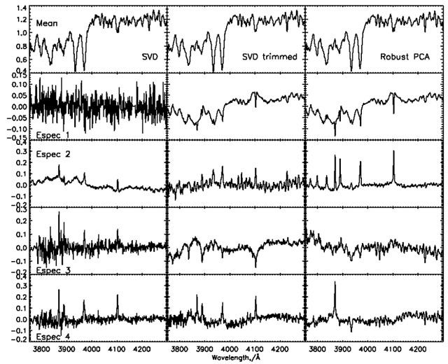Figure 10. Comparison between the eigenspectra from a PCA of 2000 randomly selected SDSS galaxies: left, using a simple SVD algorithm, the first eigenspectrum is dominated by a single noisy galaxy spectrum; center, using sigma clipping to remove outliers iteratively from the dataset, the eigenspectra are visibly less noisy; right, a robust PCA of the dataset, now the distinct patterns in the dataset are strongly visible, in particular the separation of narrow nebular emission lines from broader photospheric absorption features. [Courtesy V. Wild]

4.4. Spectral fitting by inversion

As has been mentioned in Section 2.1.1, the stellar SED of a galaxy can be represented by a sum over the SEDs of individual SSPs with appropriate weights which reflect the SFH. As long as any complications, such as dust, can be neglected this is a linear problem, i.e. a matrix inversion. More generally, inversion is the attempt to invert the observed galaxy SED onto a basis of independent components (SSPs, dust components) drawn from a SED model. Inversion is typically used for spectral data and a big success of modern stellar population models and inversion codes is that we can now fit the models to data to better than 5% in the optical wavelength range (see Section 4.4.4).

4.4.1. Method

Nearly all inversion methods start with assumptions that reduce the complex physics of SEDs (see Eq 1) to a problem that can be written as a linear function of its parameters. Such assumptions are typically that one deals with a stellar system in which all generations of stars have the same metallicity, i.e. ζ(t) = Z⁰ and the same attenuation, i.e. T(t) = T⁰. The problem of solving for the star formation history of a stellar system is then equivalent to defining and minimizing the merit function

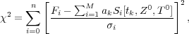(3)

over all non-negative a_k. Here F_i is the observed spectrum in each of n wavelength bins i, _i is the standard deviation and a_k are weights attributed to each of M SSP models S_i[t_k, Z] of age t_k and metallicity Z. This merit function is linear in the a_k and can thus be solved by standard mathematical methods involving singular value decomposition (e.g. non-negative least squares, bounded least squares) 3. A particular advantage of the inversion method is that, besides the assumptions necessary to linearize the problem, no parametrization of the solution is necessary, in particular not of the star formation history. Codes that have been used for scientific analysis are now common and include MOPED (Heavens et al. 2000), PLATEFIT (Tremonti et al. 2004), VESPA (Tojeiro et al. 2007), STECKMAP (Ocvirk et al. 2006), STARLIGHT (Cid Fernandes et al. 2005), sedfit (Walcher et al. 2006), NBURSTS (Chilingarian et al. (2007)), ULySS (Koleva et al. 2009). Different codes give very comparable results (e.g. Koleva et al. 2008).

There is one problem that has to be addressed when assessing the unparameterized information content of galaxy spectra. All methods relying on singular value decomposition and derived algorithms inherit one of the features, which is that the method tends to search for the smallest number of templates it can use to fit the data. For galaxies, which presumably have a smooth SFH, this feature is a grave caveat concerning the significance of the recovered weights of each population. In particular, the recovery of realistic error bars from a simple bootstrap algorithm is not possible, as the method will tend to always choose some templates over others, inside a range of random errors. One way to address this issue is regularization, detailed in Ocvirk et al. (2006, the STECKMAP program).

Another robust exploration of this issue is provided in the code VESPA (described in detail in Tojeiro et al. 2007). As independent parameters (see 4.1) Tojeiro et al. chose 2 values of metallicity and a logarithmic binning in age that can be varied between coarse (3 age bins) and fine (16 age bins). Dust attenuation and varying metallicity are explored by repeating the fit with VESPA over a grid of parameters. Error bars are derived by creating noised representations of the input spectra and repeating the fit n times. The codes main feature in the present context is that it explores the SFHs in an iterative process that goes from coarse to fine resolution. It uses the method described in Ocvirk et al. (2006) to estimate at each step, how many parameters can be recovered for a linear problem perturbed by noise. The best fit will thus only use as many independent stellar populations as required by the data. Nevertheless, one caveat remains, which is that the SFH inside each bin is fixed to be either a constant SFR or such that the light contribution of each age is more or less constant. When recovering parameters such as M/L and in those cases where the age bins are coarse, this will lead to an underestimate of the true uncertainty in this parameter, as compared to a truly non-parametric method.

The main lesson learned from this careful analysis is that from spectra typical of the SDSS (S/N 20, optical wavelength range), one can recover between 2 and 4 stellar populations described by an age and a metallicity. These values can be improved by a factor of 2 when going either from S/N = 20 to S/N = 50 or when enlarging the wavelength range to include not only the optical, but also the UV range. Such data will be available in the near future from the XSHOOTER instrument at the VLT. It should be kept in mind, however, that while the formal constraints may be better, the accuracy of the results will then depend critically on the data calibration and model accuracy over a very large wavelength range.

4.4.2. Non-linear inversion codes

For the optical wavelength range, an exception to the pre-condition of linearity exists in the form of the code STARLIGHT (Cid Fernandes et al. 2005), which is based on simulated annealing and thus does not need linearity. Consistency between STARLIGHT and other codes based on linearity assumptions has been found. Another code avoiding linearity conditions was presented in Richards et al. (2009).

For decomposing MIR spectra into their stellar, PAH, dust continuum, and line emission constituents, Levenberg-Marquardt algorithms have been used (Smith et al. 2007, Marshall et al. 2007 see Section 6.2.2) . This allows among other things to compute uncertainties on the derived parameters. With the improvement of dust emission models and in particular the more widespread availability of spectral data, more development in the technicalities of fitting dust spectra can be expected.

Finally, a possible extension of the inversion onto SSP models has been presented in Nolan et al. (2006) and would merit further exploration. Also Dye (2008) has presented a new method, which integrates inversion into a Bayesian framework and applies it to photometric data.

4.4.3. Non-linear physics

Dust attenuation is important in the optical and UV wavelength ranges. In the context of inversion, the importance of dust is most easily assessed by an iteration over a grid of attenuation values. More sophisticated schemes proceed in an iterative way, i.e. alternate linear inversion and a non-linear minimization scheme (Koleva et al. 2009), or use non-linear minimization schemes for all parameters (Cid Fernandes et al. 2005). Any estimate of the dust attenuation at optical wavelengths from the SED alone (i.e. using neither Balmer decrement, nor UV photometry, nor dust emission) is bound to be uncertain, in particular because no inversion code at present uses a physical model for different attenuations likely experienced by young and old stars.

A very useful way is therefore to normalize the continuum of the observed and model spectra before the fit (e.g. Wolf et al. 2007, Walcher et al. 2009) or even simultaneously with the fit (Koleva et al. 2009). While this takes out any information related to the attenuation, it also allows the freedom from any uncertainties related to continuum calibration and can be thought of as fitting the equivalent widths of the absorption features only. An often under-appreciated caveat is, however, that this procedure throws away some information. In particular (nearly) featureless continua (such as from very young stars) become undetectable, yet still affect the equivalent widths. This "featureless" continuum has to be appreciated in relation to the noise in the observations and, in an intermediate age spectrum can even include a significant contribution of old stars. One expression of this caveat is described in Section 4.6 as the bias occurring when fitting single SSP models to extended SFHs.

Also the effects of forward scattering on the optical SED are not included in Equation 1 and cannot be linearized usefully. In principle the scattering can be modelled through radiation transfer modelling and could thus be included in non-linear minimization schemes. However, radiation transfer modelling is too time-consuming to make this a practical possibility.

4.4.4. Validation

In an unpublished contribution to the workshop, Jarle Brinchmann (and collaborators) showed that the 10⁶ spectra of galaxies in the Sloan Digital Sky Survey (SDSS) offer a rich set of tests of the current models and techniques for fitting SEDs in the optical region. For the first series of tests they use a set of 274613 galaxies from the SDSS DR7 with reliable determinations of the emission line fluxes. They fit them using the latest version of the Bruzual and Charlot (2003) models (termed here CB08). In the optical the main improvement in these models is the switch from the Stelib library to the MILES library. The fitting procedure involves classical inversion using a non-negative least squares routine. Additionally they allow for ~ 150 Å wide mismatches between models and spectrum using a smooth final correction. This is necessary because of uncertainties in the spectrophotometry of the data and the models. The result of the NNLS routine is, among others, the mean ² of the spectrum, which can in turn be plotted into the classic (BPT Baldwin et al. 1981) diagram [N II]6584Å / H versus [O III]5007Å / H, shown in Figure 11. Generally, the fit is good, with a reduced ² around 1 ± 0.1. Regions can be identified, where the fit is, while still in this range, somewhat worse. These are (A) galaxies with high star formation activity, high excitation and low metallicity, (B) strong, high excitation AGN, and (C) galaxies with high surface mass density (i.e. high mass) and weak emission lines.

Figure 11. Classic BPT diagram of [N II] / H versus [O III] / H, showing the distribution of SDSS emission line galaxies. The colours indicate the median log 2 of the fit of the CB08 model library to the SDSS fibre spectra with those emission line ratios. The upper and lower dashed lines indicate the Kewley et al. (2001) and Kauffmann et al. (2003b) AGN dividing lines respectively. [Courtesy J. Brinchmann]

For cases (A) and (B), i.e., the low metallicity starbursts and the high-ionization AGN, they relate the main increase in ² to the imperfect masking of some emission lines and to the lack of nebular or AGN continua in the spectra. In addition the BC03 models have some problems with hot stars (e.g. Wild et al. 2007) - the preliminary version CB08 appears to work better, due to a better coverage of hot stars in the spectral library (G. Bruzual, priv. comm.).

For case (C) one of the largest mismatches in the optical is located, as expected, around the Mg features at 5100 Å. This is the region where the enhancement of the abundances of the elements is known to play an important role. -enhancement is not covered by the CB08 models. Nevertheless, in the optical the mismatch due to stellar populations is modest, of the order of 0.02 magnitudes.

The best method to validate a fitting procedure is to compare the result to independent measurements of the same physical property. This can be done for redshifts, as discussed in section 5, but also for the spectra of nuclear clusters, as done by Walcher et al. (2006) for nine nuclear clusters. The nuclear clusters have multi-aged stellar populations and are as such similar to entire galaxies, and their total stellar masses can be determined dynamically, independent from fitting the stellar spectra.. As shown in Walcher et al. (2006), the stellar M/L ratios from inversion agree with those determined from independent dynamical modelling, albeit with a large scatter. This scatter reflects the general difficulty of constraining the oldest stellar population from SED fitting. Additionally, Walcher et al. (2006) also found that the age of the youngest population as determined from the spectral fitting is correlated to the measured emission line equivalent width, as shown in figure 12 (right). On the other hand, the mean mass-weighted age is not correlated, which is evidence that the fit result is not heavily biased towards the youngest population (in contrast to results from fitting single SSPs, see section 2.1.2).

Figure 12. Comparison between the equivalent widths of emission lines and the mean age (left panel) or the age of the last burst (right panel) as determined from spectral fitting for a sample of nine nuclear clusters from Walcher et al. (2006). The clear correlation is evidence that the youngest age picked up by the spectral fit does bear significance.

Another careful work on validation of the spectral fitting procedures was the work by Koleva et al. (2008), who looked at Galactic clusters which had individual stellar spectra and full colour-magnitude diagrams to compare with the results of the fits to the integrated spectra (also compare this with section 2.1.2 for the validation of the predictions of SSP models for integrated spectra).

4.5. Bayesian inference

We refer here in particular to using the "Bayesian fitting" method, in which multi-wavelength SEDs are fit by first pre-computing a discrete set or library of model SEDs with varying degrees of complexity and afterwards determining the model SED and/or model parameters that best fit the data. This approach is favoured in particular for multi-wavelength data, as the problem of solving for the physical parameters is not linear if effects such as dust attenuation, line emission, and dust emission have to be taken into account. In addition, the influence of geometry and the physical conditions of the dust generally make the number of parameters very large, and with many possible degeneracies, thus making non-linear minimization schemes usually impractical.

4.5.1. Method

It is important to realise that the simple fact of pre-computing a set of galaxy models and afterwards determining the one with the lowest ² is by itself a Bayesian approach. By choosing which models to compute one introduces a prior, which, while possibly flat in terms of a given parameter, assumes that the data can be represented by that model and that parameter space. By using ² as a maximum likelihood estimator one finds the most probable model, or in bayesian terms, the probability of the data given that model. A mathematically much more rigorous description of the method is given in Appendix A of Kauffmann et al. (2003a) and currently builds the basis for Bayesian inference in SED fitting. A more practically oriented description can be found in e.g. section 4 of Salim et al. (2007). In a nutshell, the method uses the fact that - assuming Gaussian uncertainties - the probability of the data (D) given the model (M) is given by P(D|M) e^{-2 / 2}. The prior probability distribution of the model parameters is often taken to be flat within a given parameter range (or flat in log space for larger parameter ranges). To determine the parameters for a specific galaxy dataset, the probabilities for all models are computed and then integrated over all parameters (model space) except the one to be derived, which yields a Probability Distribution Function (PDF). The median and width of this distribution yield the parameter estimate and associated uncertainties. The integration can be repeated and the PDF can be built for all parameters of the models as well as the observables themselves, e.g. with the aim to plot the model and observed fluxes in a fitted band for comparison purposes.

An important step in Bayesian inference for SED fitting is the construction of the library and the prior assumptions (Section 4.5.2). It is equally important to synthesize the correct observables from the models, taking into account response functions and redshifts (Section 3.1).

Bayesian inference for SED fitting has several advantages that minimize potential sources of uncertainties: i) all available measurements contribute to the fit result, ii) the K-correction is integrated, iii) non-linear effects such as from dust are accounted for as part of the models (see section 2.2.2), and thus in a self-consistent way, and finally iv) uncertainties on the derived parameters include measurement uncertainties as well as intrinsic degeneracies. The big caveats concerning this method are the sensitivity to the prior distribution of parameters (the "library") and, connected to this, the dependence on realistic input physics in the modelling.

4.5.2. Libraries and priors

The computation of the library is one of the essential steps when using Bayesian inference. It encodes our prior knowledge about the galaxies in the sample, but also our assumptions about which of the physical effects we can safely neglect. Concerning photometric SEDs, a prominent case of neglection is the internal chemical evolution of the model galaxies. This is justified because even the overall metallicity is not measurable from broad-band photometry alone (e.g. Walcher et al. 2008). Also the effects of forward scattering on the optical SED are often not included for computational reasons, but could potentially be important, in particular for starbursts (Jonsson 2006).

One assumption that is generally used is that SFRs tend to decrease monotonically with cosmic time in a given object (with the exception of star formation bursts). This assumption is particularly appropriate for early-type galaxies, which has led to the wide-spread use of so-called -models, i.e. exponentially falling functions representing the SFH. However, it is not to be expected that galaxies in reality follow the falling exponential model. The SFHs of dwarf galaxies are expected to be dominated by intermittent bursts (see e.g. Gerola et al. 1980). But even for large galaxies, the SFH is not expected to be as smooth as suggested by the simple -models. Both semi-analytic (Quillen and Bland-Hawthorn 2008) and hydrodynamic modelling suggest some stochasticity, as discussed in section 4.1. However, due to the smooth variation of SED properties with age and due to the ensuing degeneracies, the -models provide reasonable fits to observed SEDs and cannot be easily refuted. Also, they provide a convenient, simple parametrization of SFHs which explains their widespread use.

The danger of using only -models lies in the neglect of degeneracies. Let us assume, the ² of a specific -model is the same as that of a different model, which is the superposition of a smooth SFH and a burst. Both models will have different mean ages and M/L ratios. If they are both included in the library, they will thus lead to a larger error bar. However, if the burst model is omitted, two situations are possible: 1) If we indeed know that strong secondary bursts are unlikely (as e.g. for a sample of morphologically selected early-type galaxies) one will obtain a better estimate of the actual error bar through use of a better prior. 2) If on the other hand one is fitting the entire population of galaxies in a given volume, it is unlikely that no galaxy shows a secondary burst and one will thus - sometimes severely - underestimate the true uncertainty of the recovered parameters. Often "new", supposedly more precise estimates of galaxy parameters are published that are based on too restrictive priors. In the following we showcase two examples of how to construct a library of star formation histories.

A library for Gaia     One of the first cases where Bayesian inference is applied to spectra will be presented in Tsalmantza, et al., (in prep). This is also a good example of how to create a library with a suitable prior for a specific application. The Gaia mission will produce spectra of 10⁶ galaxies at low resolution of R between 50 and 200. Automatic classification of a large number of low-resolution spectra is therefore crucial. Classification is done by comparison to a custom-created library of model galaxy spectra that simulate the properties of the Gaia spectra. This library is used for training and testing of the classification and parametrization algorithms.

Two libraries have been created: The first library is an entirely synthetic one. The library creation starts from the synthetic spectra of 8 typical galaxies produced by PEGASE.2 (Fioc and Rocca-Volmerange 1999). The SFHs of the library spectra are built from analytic prescriptions for either the dependence of SFR on the gas mass (SFR = M_gas^p1 / p2, late types) or for the SFH directly (SFR = p2.e^-t/p1 / p1, early types) as well as parameters for gas infall and galactic winds. In order to create a smooth grid, the input parameters (i.e. p1, p2, gas infall and galactic winds) were allowed to vary over a range of values (see Tsalmantza et al. 2007, Tsalmantza et al. 2009). At this point, while of course guided by prior knowledge of the properties of galaxies, the parameter distribution is chosen nearly ad-hoc.

A second library was created based on spectra from the SDSS (DR5, Adelman-McCarthy and et al. 2007). The SDSS spectra were shifted to z = 0 and degraded to the resolution of the PEGASE.2 output spectra. They were then classified by comparison to the pre-existing library of purely synthetic spectra through simple ²-minimization. Using the best fit model spectrum the SDSS library spectra could be extended to cover the Gaia wavelength range and values for the most significant parameters could be assigned to them. Mainly, however, the results of the ² fitting were used to judge how the synthetic library compares to the empirical galaxy population in the SDSS. The distribution of input parameters governing the SFHs obtained from the observed SDSS sample can then be used to determine a suitable prior distribution for the synthetic Gaia library. This application is a good example of a case where the prior can be well established based on other observations.

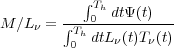
Simplifying M / L determinations     A good example of how the appropriate choice of prior can help with constraining the fit is provided by the work of Bell and de Jong (2001, and R. de Jong's talk at workshop). This work centers on finding the simplest way to derive the mass-to-light ratio of a stellar population. Let us first remember that the stellar mass itself is the product of a galaxies luminosity and its M / L. M / L in turn is a function of the star formation history of a galaxy. If the SFR at time t is written as (t) = dM(t) / dt and is defined over the entire Hubble time T_h, L(t) is the luminosity of an SSP at frequency , at age t, and with mass dM(t) and T(t) is the mean transmission of the ISM at wavelength and for the SSP with age t, then we can write

(4)

This dependence of the M / L on the SFH means that any prior assumption on the SFH is also a prior assumption on the M / L.

The crucial simplification inherent in Bell and de Jong (2001) is thus the parametrization of the SFH. This simplification is provided by a prior derived from a hierarchichal formation scenario. Using their scenario, the SFHs of galaxies lead to a situation in which their intrinsic colours show a strong correlation with M/L. The dust attenuation vector is parallel to this relation, and thus the M/L ratio can be derived from a single optical colour with reasonable precision. Nevertheless there is a curvature in the difference between the M/L ratios determined from colours only and M/L ratios determined from an SED fit in the sense that for very blue (young) galaxies and for very old (red) galaxies, the colour-M/L will provide an overestimate, while for intermediate colour, intermediate age galaxies the colour-M/L will be an underestimate.

De Jong & Bell (talk at workshop) explore different possible effects. When comparing a smooth SFH with a single burst, the M/L values have large systematic offsets, due to the lack of faint, old stellar populations in the single burst model. Two burst models do not solve the problem, in particular if the fit is dominated by two young populations. In this case the two-burst model is still not complex enough, it again misses the faint, old population, which is crucial for the mass budget. The problem with the SFH template is further clarified by a comparison between M/L ratios as determined in Bell et al. (2003a) and those derived by k-correct (Blanton and Roweis 2007). While the scatter in the difference is relatively small and there is no systematic trend, there is a systematic offset of about 0.15dex. This can traced to the parametrization of the SFH. Indeed, while Bell et al. (2003a) use pure falling exponentials, the SFH assumed in in k-correct peaks 6 Gyr after the beginning of star formation. Thus, while the resulting SED is not affected, the number of low-mass stars is much higher in the Bell et al. (2003a) SFHs. This uncertainty of 0.15 dex is thus inherent to any mass estimate from SED fitting.

4.5.3. Validation

In order to validate the method and its intrinsic accuracy, a number of studies have been performed in the last years. What could be termed "internal validation" is the search for degeneracies and systematics in the models and the method itself (see e.g. Walcher et al. 2008, Wuyts et al. 2009, Longhetti and Saracco 2009).

Extensive testing of stellar mass determinations through SED fitting was done with the COSMOS dataset (Ilbert et al. 2010). SEDs were generated with the stellar population synthesis package of Bruzual and Charlot (2003) assuming a Chabrier (2003) initial mass function (IMF) and an exponentially declining star formation history with a timescale, _*, ranging from 0.1 to 30 Gyr. The SEDs were generated on a grid of 51 timesteps between 0.1 and 13.5 Gyr. Dust attenuation was simulated using the Calzetti et al. (2000) law with E(B - V) in the range 0 to 0.5, with steps of 0.1. The colors predicted by this library of SEDs in the COSMOS dataset for the photometric redshift of the galaxy were compared to the observed ones to select the best-fitting templates.

How the potential inaccuracy of the photometric redshifts affects the stellar mass derivations was investigated, and results are displayed in Figure 13. Two spectroscopic samples were used: the zCOSMOS bright spectroscopic sample (Lilly et al. 2007) selected with a magnitude cut only at i_AB⁺ < 22.5 and a spectroscopic follow-up of 24 µm sources selected from S-COSMOS (Sanders et al. 2007). These sources are typically dusty starbursts with 18 < i_AB⁺ < 25. A median difference smaller than 0.002 dex is found between the photo-z and the spectro-z stellar masses, for both spectroscopic samples.

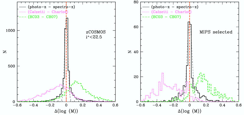Figure 13. Histograms of the difference between two stellar mass determinations, for the zCOSMOS bright sample selected at iAB+ < 22.5 (right) and for a sample of sources selected at 24 µm in the S-COSMOS MIPS sample (right). The black histograms show the difference in stellar masses when using the photometric or the spectroscopic redshifts. The thin black dashed lines are gaussian distributions with = 0.02 (left panel) and = 0.03 (right panel). The green dashed lines show the differences between the stellar masses computed with Bruzual and Charlot (2003) and Charlot & Bruzual (2007, private communication). The magenta dotted lines show the differences between the stellar masses computed using the Calzetti et al. (2000) and Charlot and Fall (2000) attenuation laws. The redshifts were set to the spectro-z values in the two last cases. Systematic uncertainties due to the models dominate the errors introduced by the photo-z, at least in the magnitude/redshift range explored with our spectroscopic samples. [Courtesy H. Aussel]

It is interesting to note that the stellar synthesis models have the same effect for both selections, as shown in Figure 13. This is not the case when studying the impact of the attenuation law. The MIPS selection consisting preferentially of dusty galaxies, the difference due to the choice of attenuation (the Calzetti et al. 2000 law in a case, the Charlot and Fall 2000 in the other) is amplified for this sample. The median difference in stellar masses is -0.1 dex for the optical selection and -0.24 dex for the infrared selection.

The impact of the choice of stellar synthesis model on the stellar masses determinations was also examined. Figure 13 presents the difference between stellar masses computed using the Bruzual and Charlot (2003) models and the new models of Charlot and Bruzual (2007, private communication) including a better treatment of the pulsing asymptotic giant branch. A median difference of 0.13-0.16 dex and a dispersion of 0.09 dex is observed. Pozzetti et al. (2007) found a similar difference (0.14 dex) when comparing Bruzual and Charlot (2003) and Maraston (2005) models. Walcher et al. (2008) show that this offset changes with the measured sSFR of the galaxy, in the sense that the masses determined using BC03 for objects with an intermediate sSFR (-12 < log(sSFR) < -9) are, in the mean, more massive by 50% than those determined using CB07. These are the objects where the TP-AGB stars are most likely to contribute significantly to the light in the NIR bands. Objects with lower or higher sSFRs do not show this offset in Walcher et al. (2008).

Ilbert et al. (2010) concluded from this study that the use of photometric redshifts is only a weak source of uncertainty when deriving stellar masses for a sample of galaxies. The uncertainties are dominated by the uncertainties in the SED modeling itself, thus one has to be very cautious about the interpretations when selecting samples where a specific type of model is preferred.

External validation of the method is possible for one parameter in particular, namely the SFR. Using the entire SED to derive the SFR was considered less precise than other methods (based on specific tracers) in Kennicutt (1998). The availability of large samples with UV, optical and NIR photometry have lead to a reappraisal of the method in the last years. Salim et al. (2007) show a detailed comparison based on the data from the SDSS and the Galex satellite. They derive SFRs using the multi-wavelength SED. They then compare these to the SFRs derived by Brinchmann et al. (2004), which used all emission lines that can be usefully measured in the SDSS spectra and detailed modelling of the emission line spectrum to derive dust-corrected, emission-line based SFRs. As shown in their figure 6, the SED-derived SFRs show in general a satisfying agreement. A similar test was performed in Walcher et al. (2008) on a VVDS-SWIRE-GALEX-CFHTLS sample, where the SED SFR was compared to SFRs derived from the [OII]3727Å emission line. While the latter are much less accurate than the emission line SFRs from Brinchmann et al. (2004), the agreement between SED and emission line SFR was shown to be satisfying out to a redshift around one (their figure 8). An advantage of obtaining SFRs from broad-band SEDs compared to emission-lines is the time needed to obtain sufficient S/N in the spectra to get the lines. Nevertheless, an interesting residual correlation of SFR difference with stellar mass is found in SED fitting, which remains yet to be fully understood. Another interesting problem exists in early-type galaxies, in which no H emission can be measured, yet UV emission is commonly found (see e.g. Salim et al. 2007, Figure 3). This probably is the cause why some objects with no measurable emission lines have relatively high SED SFRs.

In order to test the SFR determinations from SED fitting at z ~ 1, Salim et al. (2009) extended previous work to include the mid-IR dust emission. The consensus is that the mid-IR emission is heated by the UV, and hence traces the emission of young stars ( 100 Myr) and it therefore provides a good means to measure the SFR. Deep MIPS 24 µm imaging exists for the Extended Groth Strip (EGS), as well as redshifts assembled in the context of the DEEP2 survey. The rest-frame 12 µm emission was converted to a total dust luminosity using the Dale and Helou (2002) prescriptions. Using the dust attenuation determined from fitting the UV-optical SED one can calculate the dust-corrected UV and B-band luminosities. These correlate well with the 24µm luminosity as seen in figure 14. Turning the IR luminosity into a SFR using the relations of Kennicutt (1998), the best correlation was found for an SED-SFR measured over the last 1-3 Gyr. That the mid-IR may be heated by older stars recently received support in a study by Kelson and Holden (2010), which predicts that C-type TP-AGB stars ( ~ 1.5 Gyr old) can produce a large fraction of the mid-IR flux.

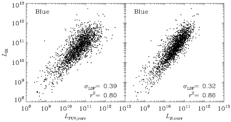Figure 14. Comparing UV and optical luminosities to the IR luminosity determined from the 24µm flux. The offset () and dispersion () around the mean relation of the galaxy sample are marked in the lower right corner. Figure from Salim et al. (2009) [Courtesy S. Salim].

Stellar mass is the second parameter that can in principle be calibrated empirically, with the hope of deriving the normalization of the M/L ratio, in other words the choice of IMF. However, uncertainties related to technical questions concerning the SED fitting and the dynamical mass measurements are still too high to derive very accurate overall IMF normalizations (see e.g. Cappellari et al. 2006, Salucci et al. 2008). Careful attention should also be paid to issues such as the contribution of dark matter, recycled gas, and other dark components. In the formulation of Bell and de Jong (2001), the slope of the colour-M/L relation is independent of the IMF, but the normalization depends on it. For this reason Bell and de Jong (2001) used the maximum disk approximation to provide an upper boundary of the total mass in stars allowed in spiral galaxies. They thus confirm that the Salpeter IMF leads to too high M/L ratios and they adapt the normalization of the colour-M/L relation to be 0.15 dex below Salpeter. Thus a Kroupa or Chabrier IMF seem to be good choices (see section 2.1.1). Variations between stellar population models and in dependence on the available data range also need to be considered carefully (see e.g. van der Wel et al. 32006). As many more independent mass tracers exist, which require careful assessment, the interested reader is pointed to de Jong & Bell (in prep.) for further discussion of this topic.

4.6. Method-independent caveats

A good example of how the quality of the available models and data influence the use of tracers and the precision with which physical properties can be recovered is given by recent developments in the use of index fitting. Historically, early-type galaxies have been analyzed using simple stellar populations models as templates, effectively using the prior assumption that early-type galaxies were created in one single burst of star formation. However, detailed spectroscopic studies (Trager et al. 2000) as well as near-ultraviolet photometry of early-type galaxies (Ferreras and Silk 2000, Yi et al. 2005, Kaviraj et al. 2007) have confirmed the presence of hot stars in early-type galaxies.

Figure 15 illustrates that it is now possible and necessary to go beyond SSPs for early-types (see also e.g. Serra and Trager 2007). The marginalized age distribution is shown for four galaxies corresponding to three different models (from left to right): Simple Stellar Populations (SSP), a 2-burst model consisting of a superposition of an old and a young SSP (2BST), and a composite model assuming an exponentially decaying star formation rate, including a simple prescription for chemical enrichment (CXP). All these models combine the population synthesis models of Bruzual and Charlot (2003). The figure shows that SSPs give mutually inconsistent age distributions, whereas composite models such as 2BST or CXP give a more consistent picture. Notice how lower mass galaxies such as NGC 4489 or NGC 4239 (top panels) give better fits for a 2 burst scenario, whereas higher mass galaxies (NGC 4464, NGC 4387; bottom panels) are better fit by a smooth star formation history.

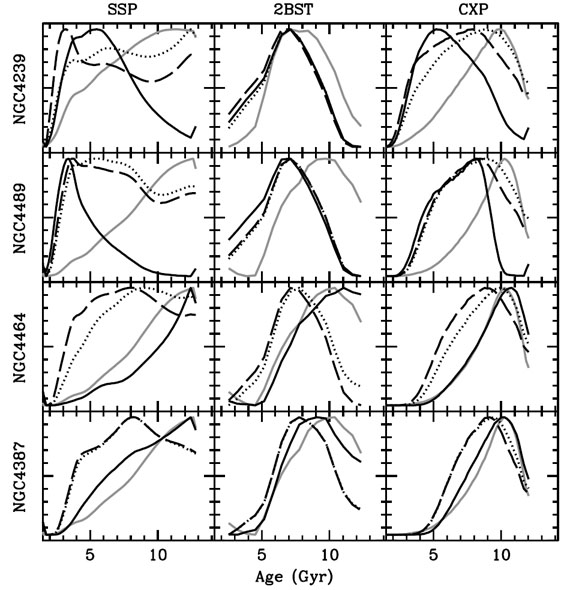Figure 15. Marginalized age distribution in four Virgo cluster elliptical galaxies. Three models for the star formation history are considered as labeled (see text for details). The black lines correspond to the age extracted from [MgFe] plus either H (solid), H (dashed) or H (dotted), respectively. The gray line is the result from the fit to the SED. [Courtesy I. Ferreras]

A similar analysis is presented in Trager and Somerville (2009), who analyze mock data from semi-analytic models in standard ways, in particular computing the "SSP-equivalent" ages and metallicities. They quantify that the SSP-equivalent age is poorly correlated with the mass-weighted or light-weighted average ages. The SSP-ages tend to be younger, biased to the star formation in the last 0.1-2 Gyr. This has in particular the effect of exaggerating the signature of downsizing. On the other hand, the SSP-equivalent metallicity is mostly equivalent to the light-weighted metallicity. This serves as an important reminder, that the prior assumption that one puts into the analysis are very important for the resulting measurement. In the case of using SSP-equivalent ages, the assumption, or prior, is that galaxies are single-age entities. This inevitably leads to important biases in the determined parameters.

Among the important caveats of SED fitting, the issue of the age-metallicity degeneracy cannot remain unmentioned. This degeneracy is particularly important in the optical. In a nutshell, age effects on colors or line strengths can be mimicked by a change in metallicity. This is especially important in the old populations found in early-type galaxies. Equally important and generally well-understood are the effects of using the optical SED only to determine the attenuation. Basically this is a very difficult undertaking and under almost any circumstance, measurements of the Balmer decrement, the FIR emission or the UV slope are essential to a reliable determination of the attenuation.

In principle it should be possible and informative to combine information from the photometric SED and spectral information (Gallazzi and Bell 2009, Lamareille 2009). While widespread use of this combination is hampered by possible systematic differences in the results (e.g. Wolf et al. 2007, Schombert and Rakos 2009), general agreement between both types of information has been claimed at least for stellar masses (Drory et al. 2004). Brinchmann et al. (Talk at workshop) showed the results of a systematic comparison between photometric and spectral SED fitting. Comparing formal errors, they find no significant systematic offset. However, for actively star forming galaxies it might be better to use multiwavelength, broad-band photometry than the detailed spectrum information. The reason is, as mentioned in Section 4.4.3, that very young stars tend to "hide" in the normalized optical part of the spectrum, however they are readily visible as blue continuum in the multi-wavelength SED. On the other hand, spectra are better at picking up recent bursts through their Balmer lines (e.g. Wild et al. 2007, Wild et al. 2009). Emission lines are a potential problem for fitting photometric SEDs. A quick back of the envelope calculation, however, shows that they produce a maximal offset in r-i colour of 0.1 at an equivalent width of 100 Å. Thus, ELs are a minor issue in the broad-band colours when a full SED is available and of limited concern for normal z ~ 0 galaxies ⁴.

Galaxies with significant redshifts can in principle be treated the same way as local ones, subject to two main caveats though: (1) we currently do not have the same kind of information available for large samples of galaxies at redshifts above 1 as for local galaxies. (2) Galaxies at high redshifts may have been significantly different from todays galaxies, e.g. concerning their typical star formation histories, their metallicities or their gas content. As local analogs are rare or lacking, SED models are less well calibrated and may be subject to considerable systematic uncertainties. These need to be explored in detail, which is currently only possible through semi-analytic models (see e.g. Schurer et al. 2009). The design limits of SED fitting codes should thus be kept in mind when quoting results and - in particular - errorbars on high redshift properties.

³ It needs to be emphasized here that a correct solution involves a simultaneous fit for the velocity dispersion of a galaxy. This is beyond the scope of the present review though. Back.

⁴ But recall that equivalent widths are proportional to (1 + z) and that the sSFR also tends to increase with redshift. Back.