


Because stellar disks contain many stars, the attraction from individual nearby stars is negligible in comparison with the aggregated gravitational field of distant matter. The Appendix explains how the usual rough calculation to support this assertion, which was derived with quasi-spherical systems supported by random motion in mind (e.g. BT08 pp. 35-38), must be revised for disks. Three factors all conspire to reduce the relaxation time in disks by several orders of magnitude below the traditional estimate (eq. A4), although it remains many dynamical times.
Fig. 1 shows the non-smooth distribution of stellar velocities of > 14000 F & G dwarf stars in the vicinity of the Sun, as found in the Geneva-Copenhagen Survey (Nordström et al. 2004, Holmberg et al. 2009, hereafter GCS). The determination of the radial velocities has confirmed the substructure that was first identified by Dehnen (1998) from a clever analysis of the HIPPARCOS data without the radial velocities (The implications of this Figure are discussed more fully in Section 10.) As collisional relaxation would erase substructure, this distribution provides a direct illustration of the collisionless nature of the solar neighborhood (unless the substructure is being recreated rapidly, e.g. De Simone et al. 2004).
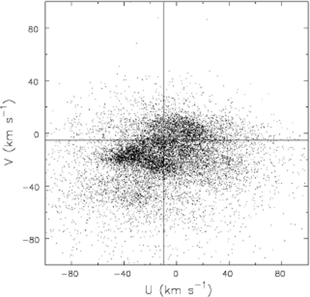 |
Figure 1. The velocity distribution, in Galactic coordinates, of stars near the Sun in the GCS. U is the velocity of the star toward the Galactic center and V is the component in the direction of Galactic rotation, both measured relative to the Sun. The intersection of the vertical and horizontal lines shows the local standard of rest estimated by Aumer & Binney (2009). |
The usual first approximation that stars move in a smooth gravitational potential well therefore seems adequate.
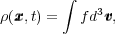
This approximation immediately removes the need to distinguish stars by their masses. A stellar system can therefore be described by a distribution function (DF), f(x, v, t)) that specifies the stellar density in a 6D phase space of position x and velocity v at a particular time t. Since masses are unimportant, it is simplest conceptually to think of the stars being broken into infinitesimal fragments so that discreteness is never an issue.
With this definition, the mass density at any point is
 |
(1) |
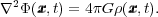
which in turn is related to the gravitational potential,
 , through
Poisson's equation
, through
Poisson's equation
 |
(2) |
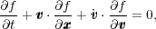
This is, of course, just the potential from the stellar component described in f; the total potential includes contributions from dark matter, gas, external perturbations, etc. Finally, the evolution of the DF is governed by the collisionless Boltzmann equation (BT08, eq. 4.11):
 |
(3) |
where the acceleration is the negative gradient of thesmooth
total potential:  = -
= - tot. The time
evolution of a stellar system is completely described by the solution
to these three coupled equations. Note that collisionless systems
have no equation of state that relates the density to quantities such
as pressure.
tot. The time
evolution of a stellar system is completely described by the solution
to these three coupled equations. Note that collisionless systems
have no equation of state that relates the density to quantities such
as pressure.
The most successful way to obtain global solutions to these coupled equations is through N-body simulation. The particles in a simulation are a representative sample of points in phase space whose motion is advanced in time in the gravitational field. At each step, the field is determined from a smoothed estimate of the density distribution derived from the instantaneous positions of the particles themselves. 1 This rough and ready approach is powerful, but simulations have limitations caused by noise from the finite number of particles, and bias caused by the smoothed density and approximate solution for the field, and other possible artifacts.
Understanding the results from simulations, or evenknowing when they can be trusted, requires dynamical insight that can be obtained only from analytic treatments. This chapter therefore stresses how the basic theory of stellar disks inter-relates with well designed, idealized simulations to advance our understanding of these complex systems.
Since orbital deflections by mass clumps can be neglected (Section 2.1), the stars in a disk move in a smooth gravitational potential. It is simplest to first discuss motion of stars in the disk mid-plane, before considering full 3D motion.
The orbit of a star of specific energy E and specific
angular momentum Lz in the mid-plane of an
axisymmetric potential is, in general, a non-closing rosette, as shown in
Fig. 2. The motion can be viewed as a retrograde
epicycle about a guiding center that itself moves at a
constant rate around a circle of radius Rg, which is
the radius of a circular orbit having the same Lz. In
one complete radial period,
 R the star advances
in azimuth through an angle
R the star advances
in azimuth through an angle

 , as drawn in the
lower panel. In fact,
, as drawn in the
lower panel. In fact, 
 2 in most
reasonable gravitational potentials;
specifically =
2 in most
reasonable gravitational potentials;
specifically =
 2
for small epicycles in a flat
rotation curve.
2
for small epicycles in a flat
rotation curve.
 |
Figure 2. An orbit of a star is generally a
non-closing rosette (upper
panel). The lower panel shows one radial oscillation, from
pericenter to pericenter say, during which time the star moves in
azimuth through the angle
|
These periods can be used to define two angular frequencies for the
orbit:  =
/ R, which is the
angular rate of motion of the guiding center, and
R =
2 /
R. In
the limit of the radial oscillation amplitude, a
=
/ R, which is the
angular rate of motion of the guiding center, and
R =
2 /
R. In
the limit of the radial oscillation amplitude, a
 0,
these frequencies tend to
, the
angular frequency of a circular orbit at R =
Rg, and
R
0,
these frequencies tend to
, the
angular frequency of a circular orbit at R =
Rg, and
R
 , the epicylcic
frequency, defined through
, the epicylcic
frequency, defined through
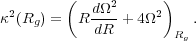 |
(4) |
If the potential includes an infinitesimal non-axisymmetric
perturbation having m-fold rotational symmetry and which turns at
the angular rate
p, the
pattern speed, stars in the
disk encounter wave crests at the Doppler-shifted frequency
m|p -
|.
Resonances arise when
 |
(5) |
where simple orbit perturbation theory breaks down for steady
potential perturbations. At corotation (CR),where
l = 0, the guiding center of the star's orbit has the same angular
frequency as the wave. At the inner Lindblad resonance (ILR),
where l = -1, or at the outer Lindblad resonance (OLR), where
l = +1, the guiding center respectively overtakes, or is
overtaken by,
the wave at the star's unforced radial frequency. Other resonances
arise for larger |l|, but these three are the most important. Note
that resonant orbits close after m radial oscillations and
l turns about the galactic center in a frame that rotates at
angular rate
p.
The solid curve in Fig. 3, the so-called Lindblad diagram, marks the locus of circular orbits for stars in an axisymmetric disk having a flat rotation curve. Stars having more energy for their angular momentum pursue non-circular orbits. The broken curves show the loci of the principal resonances for some bi-symmetric wave having an arbitrarily chosen pattern speed; thus resonant orbits, that close in the rotating frame, persist even to high eccentricities.
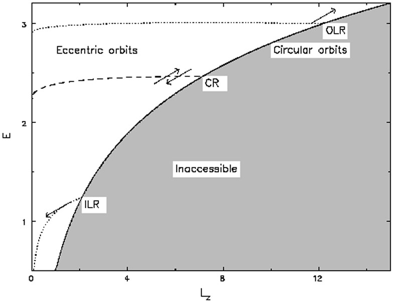 |
Figure 3. The Lindblad diagram for a disk
galaxy model. Circular
orbits lie along the full-drawn curve and eccentric orbits fill the
region above it. Angular momentum and energy exchanges between a
steadily rotating disturbance and particles move them along lines of
slope |
The arrows in Figure 3 indicate how these classical integrals are changed for stars that are scattered by a steadily rotating mild potential perturbation. Since Jacobi's invariant,
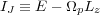 |
(6) |
(BT08 eq. 3.112), is conserved in axes that rotate with the
perturbation, the slope of all scattering vectors in
Fig. 3 is
E /
Lz
= p.
Lynden-Bell &
Kalnajs (1972)
showed that a steadily rotating potential perturbation
causes lasting changes to the integrals only at resonances. Since
c =
p at CR,
scattering vectors are parallel to the
circular orbit curve at this resonance, where angular momentum changes
do not alter the energy of random motion. Outward transfer of angular
momentum involving exchanges at the Lindblad resonances, on the other
hand, does move stars away from the circular orbit curve, and enables
energy to be extracted from the potential well and converted to
increased random motion.
Notice also from Fig. 3 that the direction of the scattering vector closely follows the resonant locus (dotted curve) at the ILR only. Thus, when stars are scattered at this resonance, they stay on resonance as they gain random energy, allowing strong scatterings to occur. The opposite case arises at the OLR, where a small gain of angular momentum moves a star off resonance.
Stars also oscillate vertically about the disk mid-plane. If the
vertical excursions are not large, and the in-plane motion is nearly
circular, the vertical motion is harmonic with the characteristic
frequency  =
(
=
( 2
/ z2)1/2, which
principally depends on the density of matter in the disk mid-plane at
Rg. As
is significantly larger than
, the frequency
of radial oscillation, the two motions can be considered to be
decoupled for small amplitude excursions in both coordinates. In
practice, the vertical excursions of most stars are large enough to
take them to distances from the mid-plane where the potential departs
significantly from harmonic (i.e. for |z|
2
/ z2)1/2, which
principally depends on the density of matter in the disk mid-plane at
Rg. As
is significantly larger than
, the frequency
of radial oscillation, the two motions can be considered to be
decoupled for small amplitude excursions in both coordinates. In
practice, the vertical excursions of most stars are large enough to
take them to distances from the mid-plane where the potential departs
significantly from harmonic (i.e. for |z|
 200 pc in the
solar neighborhood,
Holmberg & Flynn
2004).
200 pc in the
solar neighborhood,
Holmberg & Flynn
2004).
The principal vertical resonances with a rotating density wave
occur where
m(p
- )
= ± , which are at radii
farther from corotation than are the in-plane Lindblad resonances.
Since spiral density waves are believed to have substantial amplitude
only between the Lindblad resonances, the vertical resonances do not
affect density waves, and anyway occur where the forcing amplitude
will be small.
The situation is more complicated when the star's radial amplitude is
large enough that varies
significantly between peri- and
apo-galacticon. Also, the vertical periods of stars lengthen for
larger vertical excursions, allowing vertical resonances to become
important (see Section 8.1).
1 i.e. a simulation solves eqs. (1)-(3) by the method of characteristics. Back.