


Before making a direct comparison of the SBBN results, we first discuss astrophysical observations of light elements. Here we focus on 4He, D, and the Li isotopes, all of which are accessible in primitive environments making it possible to extrapolate existing observations to their primordial abundances. BBN also produces 3He in observable amounts, and 3He is detectable via its hyperfine emission line, but this line is only accessible within Milky Way gas clouds that are far from pristine [65]. Because of the uncertain post-BBN nucleosynthetic history of 3He, it is not possible to use these high-metallicity environments to infer primordial 3He at a level useful for probing BBN [66]. After an overview of the observational status of the four remaining isotopes, we turn to the CMB, which includes constraints not only on the baryon density but now also on 4He and Neff.
4He has long since been the element of choice for setting constraints on physics beyond the Standard Model. The reasoning is simple: as discussed above, the 4He abundance is almost completely controlled by the number of free neutrons at the onset of nucleosynthesis, and that number is determined by the freeze-out of the weak n ↔ p rates. The resulting mass fraction of 4He is given in Eq. (4). As we have seen, the SBBN result for the Yp dependence on the baryon density is only logarithmic and therefore 4He is not a particularly good baryometer. Nevertheless, it is quite sensitive to any changes in the freeze-out temperature, Tf, through the relation (2). However, strong limits on physics beyond the Standard Model [57] requires accurate 4He abundances from observations.
The 4He abundance is determined by measurements of He (and H) emission lines in extragalactic HII regions. Since 4He is produced in stars along with heavier elements, the primordial mass fraction of 4He, Yp ≡ ρ(4He) / ρb, is determined by a regression of the helium abundance versus metallicity [67]. However, due to numerous systematic uncertainties, obtaining an accuracy better than 1% in the primordial helium abundance is very difficult [30, 34, 68]. The theoretical model that is used to extract a 4He abundance contains eight physical parameters to predict the fluxes of nine emission line ratios that can be compared directly with observations 3. The parameters include, the electron density, optical depth, temperature, equivalent widths of underlying absorption for both H and He, a correction for reddening, the neutral hydrogen fraction, and of course the 4He abundance. Using theoretical emissivities, the model can be used to predict the fluxes of 6 He lines (relative to Hβ) as well as 3 H lines (also relative to Hβ). The lines are chosen for their ability to break degeneracies among the inputs when possible. For a recent discussion see [38, 39].
There is a considerable amount of 4He data available [33, 34]. A Markov Chain Monte Carlo analysis of the 8-dimensional parameter space for 93 H II regions reported in [34] was performed in [32]. By marginalizing over the other 7 parameters, the 4He abundance (and its uncertainty) can be determined. However, for most the data, the χ2s obtained by comparing the theoretically derived fluxes for the 9 emission lines with those observed, were typically very large (≫ 1) indicating either a problem with the data, a problem with the model, or problems with both. Selecting only data for which 6 He lines were available, and a χ2 < 4, left only 25 objects for the subsequent analysis. Further cuts of solutions with for example, anomalously high neutral H fractions, or excessive corrections due to underlying absorptions brought the sample down to 14 objects that yielded Y = 0.2534 ± 0.0083 + (54 ± 102)O/H based on a linear regression and Yp = 0.2574 ± 0.0036 based on a weighted mean of the same data.
Recently, a new analysis of the theoretical emissivities has been performed [37]. This includes improved photoionization cross-sections and a correction of errors found in the previous result. The new emissivities are systematically higher, and for some lines the increase in the emissivity is 3-5% or higher. As a consequence, one expects lower 4He abundances using the new emissivities. In [38], the same initial data were used with the same quality cuts, now leaving 16 objects in the final sample. Individual objects typically showed 5-10 % lower 4He abundance yielding Y = 0.2465 ± 0.0097 + (96 ± 122) O/H for a regression. Once again, one could argue that the lack of true indication of a slope in the data over the restricted baseline may justify using the mean rather than the regression. The mean was then found to be Yp = 0.2535 ± 0.0036. The large errors in Yp determined from the regression were due to a combination of large errors on individual objects, a relatively low number of objects with χ2 < 4, a short baseline in O/H, and a poorly determined slope (though the analysis using the new emissivities does show more positive evidence for a slope of Y vs O/H).
More recently, new observations include a near infrared line at λ 10830 [36]. The importance of this line stems from its dependence on density and temperature that differs from other observed He lines. This potentially breaks the degeneracy seen between these two parameters that is one of the major culprits for large uncertainties in 4He abundance determinations. There are 16 objects satisfying χ2 ≲ 6 [39] (there are now two degrees for freedom rather than one), with all seven He measured (though these are not exactly the same 16 objects used in [38]). Indeed it was found [39] that the inclusion of this line, did in fact reduce the uncertainty and leads to a better defined regression
 |
(7) |
Unlike past analyses, there is now a well-defined slope in the regression, making the mean, Yp = 0.2515 ± 0.0017 less justifiable as an estimate of primordial 4He. The benefit of adding the IR He line is seen to reduce the uncertainty in Yp by over a factor of two. This is due to the better determined abundances of individual objects and a better determined slope. It remains the case, however, that most of the available observational data are not well fit by the model. Comparing with the value of Yp given in Table 2, the intercept of the regression (7) is in good agreement with the results of SBBN.
Because of its strong dependence on the baryon density, deuterium is an excellent baryometer. Furthermore, since there are no known astrophysical sources for deuterium production [69] and thus all deuterium must be of primordial origin, any observed deuterium provides us with an upper bound on the baryon-to-photon ratio [70, 71]. However, the monotonic decrease in the deuterium abundance over time indicates that the galactic chemical evolution [75, 76] affects the interpretation of any local measurements of the deuterium abundance such as in the local interstellar medium [72], galactic disk [73], or galactic halo [74].
The role of D/H in BBN was significantly promoted when measurements of D/H ratios in quasar absorption systems at high redshift became available. In a short note in 1976, Adams [77] outlined the conditions that would permit the detectability of deuterium in such systems. However it was not until 1997, that the first reliable measurements of D/H at high redshift became available [78] (we do not discuss here the tumultuous period with conflicting high and low measures of D/H). Over the next 20+ years, only a handful of new observations became available with abundances in the range D/H = (1 − 4) × 10−5 [78, 79]. Despite the fact that there was considerable dispersion in the data (unexpected if these observations correspond to primordial D/H), the weighted mean of the data gave D/H = (3.01 ± 0.21) × 10−5 with a sample variance of 0.68. While the data were in reasonably good agreement with the SBBN predicted value (discussed in detail below) using the CMB determined value for the baryon-to-photon ratio, the dispersion indicated that either the quoted error bars were underestimated and larger systematic errors were unaccounted for, or if the dispersion was real, in situ destruction of deuterium must have taken place within these absorbers. In the latter case, the highest ratio (∼ 4× 10⁻⁵) should be taken as the post-BBN value, leaving room for some post-BBN production of D/H that may have accompanied the destruction of 7Li - we return to this possibility (or lack thereof) below.
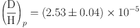
In 2012, Pettini and Cooke [80] published results from a new observation of an absorber at z = 3.05, with D/H = (2.54 ± 0.05) × 10−5 corresponding to an uncertainty of about 2% that can be compared with typical uncertainties of 10 – 20 % in previous observations. This was followed another precision observation and a reanalysis of the 2012 data along with a reanalysis of a selection of three other objects from the literature (chosen using a strict set of restrictions to be able to argue for the desired accuracy) [40]. The resulting set of five absorbers yielded
 |
(8) |
with a sample variance of only 0.05. We will use this value in our SBBN analysis below 4.
Lithium has by far the smallest observable primordial abundance in SBBN, but as we will see provides an important consistency check on the theory – a check that currently is not satisfied! In SBBN, mass-7 is made in the form of stable 7Li, but also as radioactive 7Be. In its neutral form, 7Be decays via electron capture with a half-life of 53 days. In the early universe, however, the decay is delayed until the universe is cool enough that 7Be can finally capture an electron at z ∼ 30,000 [82], shortly before hydrogen recombination! Thus 7Be decays long after the ∼ 3 min timescale of BBN, yet after recombination, all mass-7 takes the form of 7Li. Consequently, 7Li/H theory predictions sum both mass-7 isotopes. Note also that 7Li production dominates at low η, while 7Be dominates at high η, leading to the characteristic “lithium dip” versus baryon density in the Schramm plot (Fig. 1) described below.
A wide variety of astrophysical processes have been proposed as lithium nucleosynthesis sites operating after BBN. Cosmic-ray interactions with diffuse interstellar (or intergalactic) gas produces both 7Li and 6Li via spallation reaction such as pcr + 16Oism → 6,7Li + ⋯, and fusion 4Hecr + 4Heism → 6,7Li + ⋯ [83]. In the supernova “ν-process,” neutrino spallation reactions can also produce 7Li in the helium shell via ν + 4He → 3He followed by 3He+4He → 7Be + γ as well as the mirror version of these [84] though the importance of this contribution to 7Li is limited by associated 11B production [85]. Finally, in somewhat lower mass stars undergoing the late, asymptotic giant branch phase of evolution, 3He burning leads to high surface Li abundances, some of that may (or may not!) survive to be ejected in the death of the stars [86]. Thus, despite its low abundance, 7Li is the only element with significant production in the Big Bang, stars, and cosmic rays; by contrast, the only conventional site of 6Li production is in cosmic ray interactions [70, 87].
To disentangle the diverse Li production processes observationally thus requires measurements of lithium abundances as a function of metallicity. As with 4He, the lowest-metallicity data should have negligible Galactic contribution and point to the primordial abundances. To date, the only systems for which such a metallicity evolution can be traced are in metal-poor (Population II) halo stars in our own Galaxy. As shown by Spite & Spite [88], halo main sequence (dwarf/subgiant) stars with temperatures Teff ≳ 6000 K have a constant Li abundance, while Li/H decreases markedly for cooler stars. The hotter stars have thin convection zones and so Li is not brought to regions hot enough to destroy it. These hot halo stars that seem to preserve their Li are thus of great cosmological interest. Spite & Spite [88] found that these stars with [Fe/H] ≡ log[(Fe/H) / (Fe/H)⊙] ≲ −1.5 have a substantially lower Li content than solar metallicity stars, and moreover the Li abundance does not vary with metallicity. This “Spite plateau” points to the primordial origin of Li. Furthermore, the Li/H abundance at the plateau gives the primordial value if the host stars have not destroyed any of their lithium.
The 1982 Spite plateau discovery was based on 11 stars in the plateau region. Since then, the number of stars on the plateau have increased by more than an order of magnitude. Increasingly precise observations showed that the scatter in Li abundances is very small for halo stars with metallicities down to [Fe/H] ∼ −3 [89, 90, 92, 91, 93].
Recently, thanks to huge increases in the numbers of known metal-poor halo stars, Li data has ben extended to very low metallicity. Surprisingly, at metallicities below about [Fe/H] ≲ −3, the Li/H scatter becomes large, in contrast to the small scatter in the Spite plateau found at slightly higher metallicity. In particular, the trend in extremely metal-poor stars is that no stars have Li/H above the Spite plateau value, a few are found near the plateau, but many lie significantly below [95, 94]. This “meltdown” of the Spite plateau remains difficult to understand from the point of view of stellar evolution, but in any case seems to demand that at least some halo stars have destroyed their Li. Moreover, as we will see below, this possibility has important consequences for the primordial lithium problem.
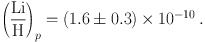
While the low-metallicity Li/H behavior is not understood, the Spite plateau remains at [Fe/H] ≃ −3 to −1.5; lacking a clear reason to discard these data, we will use them as a measure of primordial Li. Following ref. [94] we adopt their average of the non-meltdown halo stars having [Fe/H ] ≳ −3, giving
 |
(9) |
The stars in this sample were observed and analyzed in a uniform way, with Li abundances having been inferred from the absorption line spectra using sophisticated 3D stellar atmosphere models that do not assume local thermodynamic equilibrium (LTE).
Most halo star observations measure only elemental Li, because thermal broadening in the stellar atmospheres exceeds the isotope separation between 7Li and 6Li. However, very high signal-to-noise measurements are sensitive to asymmetries in the λ6707 lineshape that encode this isotope information. There were recent claims of 6Li detections, with isotope ratios as high as 6Li / 7Li ≲ 0.1 [98]. The implied 6Li/H abundance lies far above the SBBN value, leading to a putative “6Li problem.”
However, recent analyses with 3D, non-LTE stellar atmosphere models included surface convection effects (akin to solar granulation), and showed that these can entirely explain the observed line asymmetry [55, 56]. Thus case for 6Li detection in halo stars and for a 6Li problem, is weakened. Rather, the highest claimed 6Li/7Li ratio is best interpreted as an upper limit.
3.4. The Cosmic Microwave Background
The cosmic microwave background (CMB) provides us with a snapshot of the universe at recombination (zrec ≃ 1100), and encodes a wealth of cosmological information at unprecedented precision. In particular, the CMB provides a particularly robust, precise measure of the cosmic baryon content, in a manner completely independent of BBN [99, 100, 101, 102, 6]. Recently, the CMB determinations of Neff and Yp have also become quite interesting. In this section we will see how the precision of the CMB has changed the role of BBN in cosmology, and enhanced the leverage of BBN to probe new physics.
The physics of the CMB, and its relation to cosmological parameters, is recounted in excellent reviews such as [103]. Here, we briefly and qualitatively summarize some of the key physics of the recombination epoch (zrec ≃ 1100) when the CMB was released.
Tiny primordial density fluctuations are laid down in the very early universe, by inflation or some other mechanism. After matter-radiation equality, zeq ≃ 3400, the dark matter density fluctuations grow and form increasingly deep gravitational potentials. The baryon-electron plasma is attracted to the potential wells, and undergoes adiabatic compression as it falls in. Prior to recombination, the plasma remains tightly coupled to the CMB photons, whose pressure Pγ∝ T4 acting as a restoring force, with sound speed cs2 ∼ 1/3. This interplay of forces leads to acoustic oscillations of the plasma. The oscillations continue until (re)combination, when the universe goes from an opaque plasma to a transparent gas of neutral H and He. The decoupled photons for the most part travel freely thereafter until detection today, recording a snapshot of the recombining universe.
Because the density fluctuations are small, perturbations in the cosmic fluids are very well described by linear theory, wherein different wavenumbers evolve independently. Modes that have just attained their first contraction to a density maximum at recombination occur at the sound horizon ∼ cs trec. This lengthscale projects onto the sky to a characteristic angular scale ∼ 1∘; this corresponds to the first and strongest peak in the CMB angular power spectrum. Higher harmonics correspond to modes at other density extrema. The acoustic oscillations depend on the cosmology as well as the plasma properties, which set the angular scales of the harmonics as well as the heights of the features, as well as the correspondence between the temperature anisotropies and the polarization. This gives rise to the CMB sensitivity to cosmological parameters.
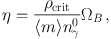
Precision observations of CMB temperature and polarization fluctuations over a wide range of scales now exist, and probe a host of cosmological parameters. Fortunately for BBN, one of the most robust of these is the cosmic baryon content, usually quantified in the CMB literature via the plasma (baryon + electron) density ρb written as the density parameter Ωb ≡ ρb / ρcrit where the critical density ρcrit = 3H02 / 8π G, with H0 = 100 h km s−1 Mpc−1 the present Hubble parameter. This in turn is related to the baryon-to-photon ratio η via
 |
(10) |
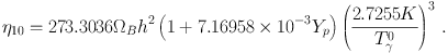
where nγ0 = 2ζ(3) T03 / π2 is the present-day photon number density. The mean mass per baryon ⟨ m ⟩ in eq. (10) is roughly the proton mass, but slightly lower due to the binding energy of helium. As a result, the detailed conversion depends very mildly on the 4He abundance [104], and we have
 |
(11) |
The CMB also encodes the values of Yp and Neff at recombination. The effect of helium and thus Yp is to set the number of plasma electrons per baryon. This controls the Thomson scattering mean free path (σT ne)−1 that sets the scale at which the acoustic peaks are damped (exponentially!) by photon diffusion. The effect of radiation and thus of Neff is predominantly to increase the cosmic expansion rate via H2 ∝ ρ. This also affects the scale of damping onset, when the diffusion length is comparable to the sound horizon [105]. Thus, measurements of the CMB damping tail at small angular scales (high ℓ) probe both Yp and Neff. In fact, the CMB determinations of these quantities are strongly anticorrelated–a higher Yp implies a lower diffusion mean free path, which is equivalent to a larger sound horizon ∼ ∫da / a H and thus lower Neff.
Since the first WMAP results in 2003 [99] sharply measured the first acoustic peaks, the CMB has determined η more precisely than BBN. Moreover, both ground-based and Planck data now measure the damping tail with sufficient accuracy to simultaneously probe all of (Ωb h2, Yp, Neff) [6, 106, 107]. Of course, BBN demands an essentially unique relationship among these quantities. Thus, it is now possible to meaningfully test BBN and thus cosmology via CMB measurements alone!
We adopt CMB determinations of (Ωb h2, Yp, Neff) from Planck 2015 data, as described in detail below, Section 4.3. We note in passing that these CMB constraints rely on the present CMB temperature, Tγ0, which is held fixed in the Planck analysis we use. In the future, Tγ0 should be varied in the CMB data evaluation, in order to provide the most stringent constraint on the relative number of baryons in the universe.
3 Below, we will use results based on the inclusion of a tenth line (seventh He line) seen in the near infra-red [36]. Back.
4 Note that the most recent measurement described in [81] has a somewhat larger uncertainty, and its inclusion does not affect the weighted mean in Eq. (8) Back.