3. SHAPE CORRELATIONS

The average shear and intrinsic alignment signal should vanish on very large scales because of statistical isotropy of the Universe. However, both effects cause local coherent variations in observed ellipticity that can be used to measure cosmic shear and intrinsic alignments over a range of scales. In this section we will introduce some of the statistics used to describe these correlations and measure them in data.

Both weak gravitational lensing and intrinsic alignments produce a correlation between galaxy shape and matter density. In addition to observed galaxy ellipticity, it is useful to consider another quantity, the projection of the ellipticity of a galaxy perpendicular to the line connecting the position of that galaxy to some point. This is called the tangential shear, γ₊, and is related to the observed ellipticity parameters through

(12)

where ϑ_P is the position angle with respect to the centre of the lens. The sign convention in Equation 12 is such that γ₊ < 0 implies tangential alignments while γ₊ > 0 implies radial alignments. As an example, tangential shear is important in determining the masses of galaxy clusters (Okabe et al., 2010, Applegate et al., 2014, Hoekstra et al., 2015), where ensemble-averaged tangential shear as a function of cluster-centric radius can be related to the projected mass, or fit by a parametric model for the mass distribution (see Hoekstra et al., 2013, for a recent review).

In this section we will concentrate on the most frequently used statistics in the intrinsic alignment literature: two-point correlations over large scales. These are particularly relevant for the large-scale measurements presented in Section 4 and for understanding the impact of intrinsic alignments on cosmic shear surveys detailed in Section 6. For more detail on environment-dependent measurements see Section 5 and some discussion of higher-order statistics can be found in Section 6.5.

In Section 3.1 we introduce the relevant two-point correlation functions before describing practical estimators for the same correlation functions in Section 3.2. In Section 3.3 we describe the projection of three-dimensional statistics along the line of sight before relating these observables to intrinsic alignment models in Section 3.4. In Section 3.5 we describe some common systematic and null tests used when making measurements of intrinsic alignments.

3.1. Two-point correlation functions

If the density or ellipticity (or shear) field is Gaussian, then all the cosmological information is contained in the correlations between galaxy positions, galaxy shapes, and the (cross-)correlations between positions and shapes, averaged over pairs of galaxies as a function of separation. These are known as two-point correlation statistics. If redshift information is available, the correlations can be computed for galaxies binned in redshift. This allows the calculation of auto- and cross-correlations of redshift bins. This is referred to as a tomographic analysis. In the case of non-Gaussian fields, due, for instance, to non-linear structure formation on small scales, higher-order statistics, such as the bispectrum, can be used to extract further information.

The statistical properties of the projected mass distribution are most easily quantified using the correlations between galaxy shapes as a function of their separation, i.e. in configuration space. This approachs allows for the treatment of complicated masks and survey boundaries. The corresponding ellipticity autocorrelation function is defined as the excess probability that any two galaxies are aligned (with respect to some arbitrarily defined coordinate system):

(13)

where i, j ∈ {1,2} denote pairs of galaxies and the angle brackets represent averaging over all pairs separated by angle θ = |θ|. Because of parity the correlation vanishes if i ≠ j and isotropy ensures that the correlation function is a function only of the separation |θ| for i = j.

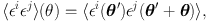
Equation (13) is defined with reference to (local) coordinate axes which are somewhat arbitrary. Instead it is more convenient to consider the ellipticities with respect to axes oriented tangentially (+; see Equation (12)) or at 45 degrees (×) to a line joining each pair of galaxies. For convenience, it is common to define the ellipticity correlation functions

(14)

We note that this notation is used in cosmic shear studies, but that it is different from the conventions commonly used in clustering studies, where the symbol ξ indicates the correlation function in 3D, and w is used for projected quantities. We will try to clarify these differences where needed.

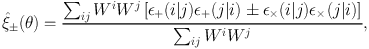
When ellipticity correlation functions are estimated from real, noisy data, a weighted combination of observed ellipticities is employed:

(15)

where the weight W_i typically accounts for the measurement uncertainties and we use є₊(i|j) to mean the + component of the ellipticity of a galaxy i, measured relative to the vector linking it to galaxy j, є_×(i|j) is te same for the × component. In the absence of intrinsic correlations these estimators are unbiased tracers of the weak lensing shear correlation functions, ⟨ є₊(i|j)є₊(j|i) ± є_×(i|j)є_×(j|i)⟩ = σ_є²δ_ij + ξ_±(|θⁱ − θ^j|), where δ_ij is the Kronecker delta and the angle brackets indicate an ensemble average over the intrinsic ellipticity distribution and over the cosmic shear field, assuming randomly-oriented intrinsic ellipticities (Schneider et al., 2002a). Though of course, due to intrinsic alignments, this is not the case in reality.

The ellipticity correlations between galaxies with similar redshifts can be used to determine the II signal: correlating the shapes of physically close galaxies boosts the intrinsic alignment signal, compared to the gravitational lensing contribution. This requires very good redshift information for the sources, and even in this case the observed signal contains a contribution from gravitational lensing itself, unless one restricts the analysis to z ≲ 0.1, where the lensing signal is very small (Heymans & Heavens, 2003). Alternatively one can remove such close pairs from the lensing analysis, thus efficiently suppressing the II contribution.

The GI contribution, on the other hand, cannot be easily removed as it results in correlations between the shapes of galaxies that are separated in redshift. To estimate the GI signal, we need to determine the cross-correlation of galaxy ellipiticity with the matter overdensity, ξ_{δ +}(r_p, Π, z), or its projection, w_δ+(r_p). The subscript δ+ indicates that we are correlating the density δ with the tangential ellipticity є₊ for pairs separated by a transverse separation r_p and a radial distance Π along the line of sight. In general it is not possible to directly estimate the matter overdensity field, δ, because the bulk of the matter in the Universe consists of dark matter. Instead galaxies are used as (biased) tracers of the density field. The cross-correlation of galaxy position with ellipticity is indicated by ξ_g+(r_p, Π, z). A positive ξ_g+(r_p, Π, z) is a signal of coherent radial alignments of galaxy ellipticity with galaxy density. Assuming galaxy density traces the matter density, this is the correlation which sources intrinsic alignments of galaxy ellipticity, in both the II and GI flavours. Negative ξ_g+(r_p, Π, z) indicates tangential alignments induced by gravitational lensing. See Equation (18) for a practical estimator of this correlation.

The shear field can be decomposed into a gradient and a curl component. The curl-free component is commonly referred to as the “E”-mode, whereas the pure curl component is called the “B”-mode, analogous to the polarisations of the electric and magnetic field.

If weak gravitational lensing was the only source of correlations in the shapes of galaxies, then one would expect to observe ξ_BB(θ) = 0. Although this is a good assumption for current surveys, a number of effects can introduce B-modes. For instance, Schneider et al. (2002b) showed that B-modes are introduced if the source galaxies are clustered. However, most of these effects are expected to be small, and the measurement of the B-mode has been used as a measure of residual systematics (as instrumental effects tend to include B-modes). However, intrinsic alignments can also introduce B-modes. Both the linear and quadratic alignment models are believed to source B-modes (Hirata & Seljak, 2004), while Crittenden et al., (2001) and Crittenden et al., (2002 showed that spin alignments are not curl-free. Although the level of B-modes remains uncertain, it is too small to be detected in current surveys.

3.2. Estimators of the two-point correlation functions

The ellipticity correlation functions are straightforward to compute from observations and are insensitive to the survey geometry. This geometry is usually rather complex because of areas that need to be masked due to the presence of bright stars or other artefacts in the data and must be accounted for when estimating the galaxy correlation function ξ_gg. Nonetheless, it is important that the estimator that is employed accounts for the fact that some measurements are noisier than others. Alternatively, one may want to define estimators that minimise certain biases. In practice the correlation functions are computed from entries in a galaxy catalogue, which lists their positions, shapes, etc.

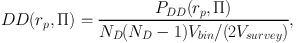
Assume that D is a catalogue of N_D galaxies with positions from which we can compute P_DD(r_p, Π), the number of pairs as a function of separation. It is convenient to normalise the result by the total number of pairs, given by N_D(N_D − 1)/2, and the volume fraction, to define:

(16)

where V_survey is the total volume of the survey and V_bin is the volume of some three-dimensional bin in r_p and Π. The volume of the bin is given by V_bin = 2 π r_p Δ r_p Δ Π, in the limit that Δ r_p is small. If the galaxies are clustered then DD will be larger than unity on small scales. If we were considering a cross-correlation, rather than an auto-correlation, the equivalent normalisation would be N_D1 N_D2 V_bin / V_survey.

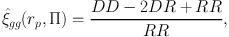
However, we have not so far taken into account the survey geometry. The simplest way to do this is to consider a catalogue of objects with random positions, but to which the mask has been applied. This random catalogue is indicated by R and should contain many more entries than the data to avoid introducing unnecessary noise. RR denotes a pair of galaxies where both are drawn from the random catalogue. The most commonly used estimator for modern studies is the Landy-Szalay estimator (Landy & Szalay, 1993). For the galaxy position auto-correlation this takes the form:

(17)

where DR means a pair of galaxies with one drawn from the data and one from the random catalogue.

A version of this estimator can be adopted for the GI cross-correlation function. In this form it is referred to as the modified Landy-Szalay estimator (Mandelbaum et al., 2011):

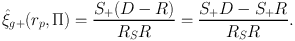(18)

Here we have assumed that, as well as the galaxy population, D, we have some other set of galaxies, S, with good shape measurements (note these could be the same population, or S could be some sub-set of D). R and R_S are now sets of random positions corresponding to the position sample and shape sample respectively. S₊D is the sum of the + component of the ellipticity over all pairs of galaxies with separations r_p and Π, where one galaxy is in the good shape sample and one is in the position sample,

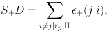(19)

for a pair of galaxies i and j. Similarly we can define the estimators for the tangential and cross ellipticity autocorrelations,

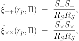(20) (21)

where

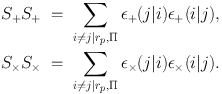(22) (23)

Alternatively one can define correlation functions of spin or position angles but, as mentioned earlier, a direct relation to the ellipticity correlation function then requires knowledge of the underlying ellipticity distribution. Hence, to be useful to mitigate the impact of intrinsic alignments in weak lensing studies, shapes need to be measured regardless.

3.3. Projected correlation functions

Although three-dimensional correlation functions are conveniently computed from theory, the observations are most commonly presented as projected quantities. Here we describe the projection of a general correlation function but it applies specifically to each of the correlations described above.

Consider a three-dimensional correlation function, ξ_ab(r_p, Π, z), where the separation of our pair, ab, under consideration has been split into components parallel, Π, and perpendicular, r_p to the line of sight. The presence of z is because the correlation function itself may depend on redshift. The corresponding projected correlation function, w_ab(r_p), for objects in a particular redshift bin, separated by a distance r_p, transverse to the line of sight, is obtained by integrating the equivalent 3D correlation function ξ_ab(r_p, Π, z) along the line-of-sight:

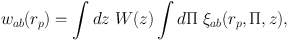(24)

where Π is the distance along the line of sight coordinate, and W(z) is the redshift weighting (Mandelbaum et al. 2011),

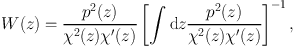(25)

where p(z) is the unconditional probability distribution of galaxy redshifts. a, b represent any combination of observables, a, b ∈ {δ, g, є, +, ×}, where δ is the matter overdensity, g is galaxy position, є is galaxy ellipticity and +, × are the components of ellipticity parallel/perpendicular or at 45^∘ to the vector connecting the pair of positions. If redshift information is available, it is convenient and straightforward to express the measurements as a function of r_p in physical coordinates. Alternatively one can show results as a function of angular separation, although this only applied to early results in practice.

The most precise results are obtained if spectroscopic redshifts (Appenzeller 2013) are available. However, this requires relatively large investments of observing time on large telescopes, especially for the faint galaxies typically used in weak lensing studies. Alternatively we can use photometric observations in multiple filters which probe features in the spectral energy distribution, which in turn can be used to estimate a photometric redshift (see e.g. Hildebrandt et al. 2012, for their application to the CFHTLenS dataset). Compared to spectroscopy, photometry is less precise but faster and therefore cheaper. Most of the observations discussed here use spectroscopic redshifts but the larger number density available from photometric surveys makes their use desirable, even at the cost of lower redshift accuracy.

Unsurprisingly the photometric redshift scatter tends to smear the intrinsic alignment signal along the line-of-sight direction, Π (Joachimi et al. 2011). When calculating projected two dimensional correlation functions, the full intrinsic alignment signal can be retained by extending the range of Π considered in a measurement. This does however reduce the measured signal-to-noise ratio, because the signal has become more spread out, and increases the contamination by gravitational shear. In practice the line-of-sight integral gets truncated and some portion of the intrinsic alignment signal is lost. This effect can be seen in Figure 2. In the lower panel, where exact redshift information is assumed, the power of the galaxy position-ellipticity correlation falls off very quickly with line-of-sight separation. In the upper panel, where a Gaussian photometric redshift scatter of width σ_z = 0.02 is assumed, there is still significant correlation, even at line-of-sight separations of > 100 Mpc / h.

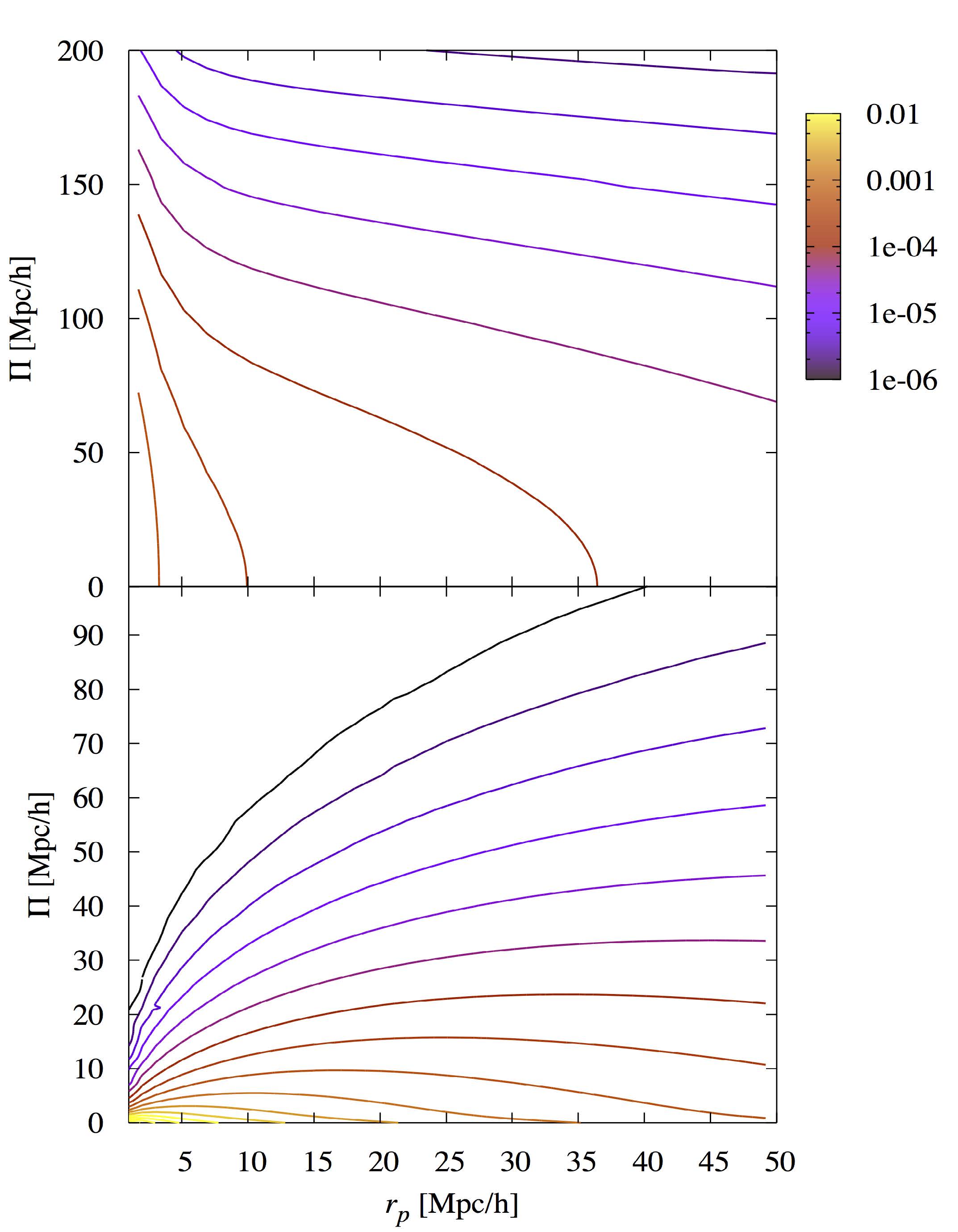Figure 2. Three-dimensional galaxy position-ellipticity correlation function, ξg+(rp, Π), as a function of comoving line-of-sight separation Π and comoving transverse separation rp at z ∼ 0.5. Contours are logarithmically spaced between 10−2 (yellow) and 10−6 (black) with three lines per decade. Top panel: Applying a Gaussian photometric redshift scatter of width 0.02. Bottom panel: Assuming exact redshifts. Note the largely different scaling of the ordinate axes. The galaxy bias has been set to unity, and the linear alignment model with SuperCOSMOS normalisation (see Section 4) has been used to model Pδ I in both cases. Redshift-space distortions have not been taken into account. Reproduced with permission from Joachimi et al. (2011) © ESO.

3.4. Using correlation functions to test intrinsic alignment models

A detailed physical understanding of our measurements requires comparison with theoretical alignment models, such as the ones that are detailed in Kiessling et al. (2015). From a theory perspective, it is often more convenient to calculate correlations in Fourier space or in spherical harmonic space. The resulting power spectrum can be directly related to the real space statistics, however the choice of space for the measurement can depend on the survey geometry (e.g. for a wide-field survey a spherical harmonic expansion is natural on the sphere), or related to the strength of the signal (e.g. the presence of bad pixels mean configuration space can be preferred), or on the numerical tools available. In this section we will concentrate on the galaxy-ellipticity correlation but the relations generalise to other observables, see Kiessling et al. (2015) for the full range of expressions.

We can relate the projected galaxy position-ellipticity correlation function, w_g+(r_p), directly to the three-dimensional density-intrinsic ellipticity function in Fourier space, P_{δ I}(k_⊥, z), via

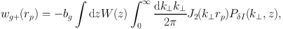(26)

where b_g is the galaxy bias, J₂(k_⊥ r_p) is the second-order Bessel function of the first kind, k_⊥ is the wavevector perpendicular to the line-of-sight and W(z) is the weighting over redshifts as derived by Mandelbaum et al. (2011), see Equation (25).

The contribution from intrinsic alignments is encoded in the three-dimensional power spectrum P_{δ I}(k_⊥, z). One model we will refer to throughout this paper is the linear alignment model (Hirata & Seljak 2004),

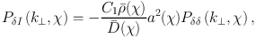(27)

where C₁ is a constant setting the amplitude of correlation, ρ(χ) is the mean matter density of the Universe, D(χ) = D(χ)(1 + z), D(χ) is the linear growth function, a(χ) is the scale factor and P_{δ δ}(k_⊥, χ) is the linear matter power spectrum. We refer to Kiessling et al. (2015) for more information on this and other specific models. We can also construct projected angular correlation functions, C(ℓ), directly from the three-dimensional power spectra, see Section 6 for more details.

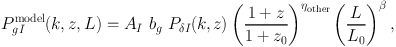
There are no explicit dependencies on redshift or galaxy luminosity in the linear alignment model but it is often thought useful to check for these when fitting to data. This is because the strength of coupling between dark matter and galaxies is unknown. These extra terms help describe the dependence of the coupling. A common approach in the literature is to insert power-law dependences on redshift, z, and the luminosity, L, where the index of the power-law is a free parameter that can be fit to data. Putting these together produces a model of the form

(28)

where P_{δ I} is the power spectrum for the mass density - intrinsic ellipticity correlation, provided by some intrinsic alignment model. A_i is a free amplitude term, b_g is the (linear, deterministic) galaxy bias, z₀ is a reference pivot redshift, L₀ is a reference pivot luminosity and η_other, β are the free power-law indices for the redshift and luminosity dependence respectively. The power-law index for redshift has been called η_other because it attempts to capture redshift evolution due to any “other” physical processes beyond the linear alignment model.

3.5. Tests for systematics

Some of the correlations are expected to be consistent with no signal in the absence of systematics errors. Such null tests can be used to test for the presence of systematics in the data, and a significant detection of a signal is a warning that the measurements of real interest may be biased. For instance, we already saw that the ellipticity auto-correlations can be written in terms of curl-free “E” and divergence-free “B” modes. Although the signal caused by spin alignments is not curl-free, the much stronger signal from the linear alignment model as well as weak lensing itself comprise only E-modes to first order. Therefore such a decomposition can be a useful diagnostic in studying the effects of systematics, even though the B-mode signal is not expected to vanish completely.

A common null test in the literature is the measurement of w_g×, the correlation of the density sample with the cross-component of the shear from the shape sample, i.e. the ellipticity measured at 45^∘ to the line connecting the pair of galaxies under consideration, one from the shape sample, the other from the density-tracer sample. This statistic is of course very closely related to the measurement of w_g+, the correlation of the density sample with the ellipticity measured along the connecting vector, and requires no additional data products, random catalogues or statistical tools. Parity symmetry means w_g× is expected to be zero. A non-zero measured value might indicate the presence of a range of systematic effects including residual PSF distortions. The cross-component of the shear is useful generally as a systematic. Another related statistic is w_+×, which is expected to be consistent with zero in the absence of systematics because intrinsic alignments only induce alignments in the radial/tangential direction.

A different null test is the calculation of w_g+, the same statistic used to measure shape alignment, but where only certain pair separations are considered. The chosen scales should be such that this correlation function will vanish because the line-of-sight separation is sufficiently large that intrinsic alignments are negligible, being a local effect, but small enough that gravitational lensing shear is still negligible. Spurious galaxy alignment, whether from optical distortion in the telescope, deblending, mistaken sky subtraction or photometric redshift errors could generate a w_g+ signal at large (apparent) separation.

These various tests were applied to the observational results that are reviewed in more detail in the next few sections. Many of these studies found w_g+ consistent with zero at large line-of-sight separation, and w_g× consistent with noise at all scales (e.g. Hirata et al., 2007, Mandelbaum et al., 2011, Joachimi et al., 2011, Singh et al., 2014)). While as yet undiscovered systematic effects cannot entirely be ruled out, these results give us hope that the intrinsic alignment signal can be reliably determined from current and near-future data.

Multiple shape measurement codes can be applied to the same data. Of course common systematic effects will manifest in both the resulting shape catalogues, but any method-specific systematics can be detected by looking at differences in correlations using the different shape estimates. For example, Sifón et al. (2015) shows results using two different shape measurement pipelines for this reason.