Copyright © 2013 by Annual Reviews. All rights reserved
| Annu. Rev. Astron. Astrophys. 2013. 51:63-104
Copyright © 2013 by Annual Reviews. All rights reserved |


A general analytical solution of the stationary 3D dust RTE is not possible for any of the non-symmetric applications mentioned in the introduction. To apply numerical solution techniques, solvers generally discretize the solution vector or the physical properties in the RTE. The quantities requiring discretization are the three spatial coordinates, the two directional coordinates, the wavelengths, and/or the dust properties.
A major concern when solving a 6D integro-differential equation is the size of the solution vector. With a resolution of 100 points in each variable, the intensity vector has 1012 entries. Handling this intensity vector requires an enormous amount of computer memory and speed. Currently, many solution algorithms avoid this requirement by not storing the full solution vector. There are applications for which the full direction-dependent intensity is needed (e.g., when the radiation pressure impacts the gas kinematics). Due to this high dimensionality of 3D RT, the choice of appropriate grids is mandatory to effectively apply existing solution techniques and minimize memory usage and runtime. The solution techniques used do influence the choice of grids (e.g., RayT versus MC).
Another concern is that for a discrete solution vector, the physics is only solved at the grid resolution, even if the solver used has no intrinsic error. Thus, if the grid is too coarse, a strong change in the intensity due to a change from optically thick to thin media may not be resolved, and the derived intensity would have large systematic errors. This makes the choice of grid crucial.
For many astrophysical applications, the density values cover orders of magnitudes and are highly structured (e.g., a turbulent gas cloud with filaments and shocks). The same is true for sources such as dust grain emission, the distribution of stars, or a layer within a photon dissociation region (PDR) emitting in the MIR. Consequently, the complexity of spatial grids in 3D continuum RT ranges from simple linear Cartesian grids (Stenholm, Stoerzer & Wehrse 1991) to adaptively refined Cartesian grids (Kurosawa & Hillier 2001, Niccolini & Alcolea 2006, Lunttila & Juvela 2012) to multiwavelength adaptive mesh refinement (AMR) grids (Steinacker, Bacmann & Henning 2002). Figure 2 illustrates complex dust distributions for three different cases using refined Cartesian grids. In principle, the RTE could be solved on unstructured, dynamic grids such as those used in line RT (Petkova & Springel 2011, Paardekooper, Kruip & Icke 2010). Finally, an analytical formula could provide the density or source distribution.
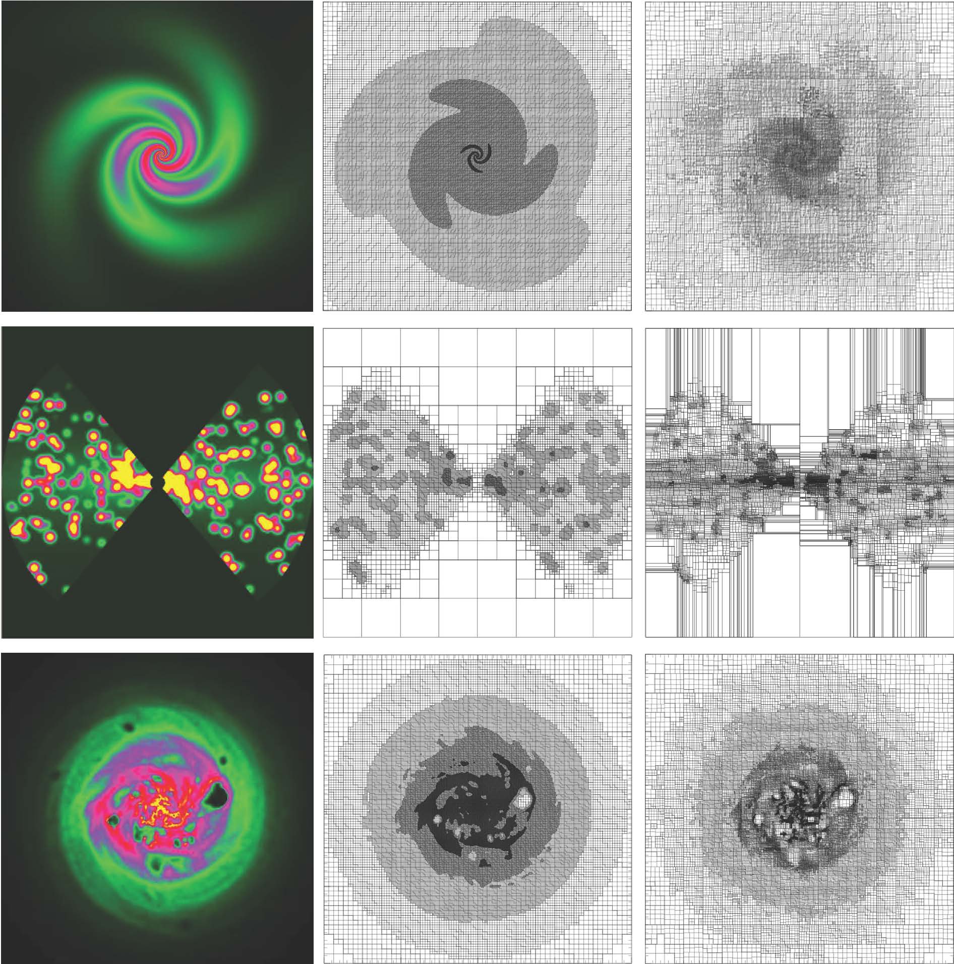 |
Figure 2. Examples of advanced spatial grids used currently for three-dimensional (3D) dust radiative transfer calculations (Saftly et al. 2013). The panels are 2D plane cuts through octree-based grids used in Monte Carlo simulations; similar grids are applied in ray-tracing techniques. The left-most panels of each row show the dust density, the central panels the grid distribution in a regular octree structure, and the right-most panels the grid distribution in a barycentric octree structure. The top row represents a regular, analytical model of a double-exponential disc with a three-armed logarithmic spiral density perturbation. The middle row corresponds to a clumpy active galactic nuclei model consisting of several optically thick clumps in a smooth density distribution (Stalevski et al. 2012). The bottom row corresponds to a late-type disc galaxy model resulting from N-body/smoothed-particle hydrodynamics simulations with strong supernova feedback (Rahimi & Kawata 2012). In all cases, the grids contain between 3 and 4 million cells. |
The optimal grid would be based on changes in radiation field intensity. As we do not know the radiation field a priori (this is the goal of the RT calculations), it is extremely challenging to generate such an optimal grid. First, the spatial grid is only 3D, whereas the intensity is defined in 6D (spatial, direction, and wavelength). For example, the intensity in a certain direction can remain constant between two positions, while the intensity in another direction can vary drastically between the same positions. The radiation field also depends on the wavelength, so the optimal spatial grid is different for each wavelength. The dust mass density, or the optical depth, could serve as the starting point on which the grid could be based (see, e.g., Figure 2, which shows 3D RT octree grids with a refinement criterion based on the total dust mass in a cell). However, the cells optical depth alone is not suitable to define a grid refinement criterion, as the strength of the radiation field can show strong gradients even in regions where the optical depth is small. In summary, the optimal grid should combine the distribution details of both the dust and source terms such that it captures the variation of the radiation field intensity.
Various approximations are used, given the difficulty in creating an optimal spatial grid. To review the variety of grids and their purposes, it is constructive to distinguish three spatial grid classes. They are used in various combinations by different solvers and in the different astrophysical communities.
3.1.1. LOCAL MEAN INTENSITY STORAGE GRIDS This most common class of grids stores the mean intensity with the goal of resolving its variation. In the end, the grid's resolution determines the spatial resolution of the obtained solution.
To achieve a reasonable sampling of the gradients in the mean intensity, it is possible to calculate a series of spatial grids that are refined using the local optical depth averaged over all directions for each wavelength. The computational effort to calculate such grids is negligible compared to the effort of solving the RTE (Steinacker, Bacmann & Henning 2002). The drawback of multiwavelength grids is that many interpolations have to be performed to assemble the wavelength-dependent radiation field. Such interpolations are time consuming and introduce interpolation errors. As a compromise, grids optimized for tracking the variation in the local optical depth for the wavelengths that dominate the radiative energy locations can resolve the important regions at the expense of excess grid points. Niccolini & Alcolea (2006) proposed an alternative way of building the grid in which an initial calculation defines the explicit locations of several photons, which are then used to refine the grid to have a constant absorption rate in each grid cell.
3.1.2. DENSITY AND SOURCE GRIDS The grids storing density and source information can originate from a discretization of simple physical models to deep structure grids designed to resolve the kinematic processes. Common examples of the latter are the AMR grid and smoothed-particle (SP) distributions used in hydrodynamical simulations (see, e.g., Steinacker et al. 2004), which typically incorporate several tens of millions of cells and many levels of refinement or smoothed-particle hydrodynamics (SPH) particles. Although RT calculations can be performed directly using such density grids (Abel & Wandelt 2002), in most cases the density information is stored on coarser grids to meet the storage and speed limitations of the 6D RT.
3.1.3. SOLUTION GRIDS The third class of grids is designed to calculate the solution directly at the grid points by advancing from one cell to the next in one step. The refinement criterion is defined to minimize solution errors of a certain order (Steinacker et al. 2002) or to provide a flexible grid that minimizes solution errors due to the coarse spatial coverage of the physical quantities (Paardekooper, Kruip & Icke 2010). These grids are well suited for MHD codes. Solving the RTE directly on a grid accumulates discretization errors causing, in the case of finite-differencing solvers, for example, a smearing of beams. Additional numerical methods or higher-order corrections compensate for these numerical diffusion errors. In some applications, the source function may also contain a smaller number of discrete sources such as stars. These can be considered outside the main spatial grid or by using smaller subgrids (Stamatellos & Whitworth 2005).
There are two major challenges in defining a fixed direction grid for 3D RT. First, the radiation field can be strongly peaked due to nearby sources, and a smearing of this beam due to insufficient direction resolution will result in remote regions not being illuminated accurately. Because the optimal intensity discretization can vary greatly across the domain, a globally optimal refinement of direction space is not usually possible. Second, even direction grids optimized to be equally spaced on the unit sphere (Steinacker, Thamm & Maier 1996) require many points to provide good angular resolution. The HEALPix method, which subdivides the unit sphere in pixels of equal size, offers another possible regular direction grid (Górski et al. 2005). For example, a grid with 600 direction points equally spaced on the unit sphere provides a mean resolution of ~ 10° only, and it takes 10,000 grid points to achieve a mean resolution of ~ 2.5°. For a protoplanetary disk, this resolution corresponds to a 4-AU hot dust region placed at a distance 100 AU from the central star.
The two main RT solution techniques treat the discretization of directions quite differently. In MC, the direction of the photons is not discretized but sampled from a probability function. For example, the calculation of the scattered intensity in MC is based directly on the scattering phase function, allowing an arbitrarily precise solution. In RayT, a discrete direction grid is used for all calculations. The scattered intensity calculation is done on the direction grid, potentially undersampling the scattering process in the direction space of the solution.
Another issue in direction space is the divergence of rays or photon tracks. The chance to miss physically important parts of the domain increases with the distance from the current point or cell. When tracing the radiation from a single source, this can lead to large errors in the computed radiation field for distant cells, or long runtimes to increase resolution using more photons or rays. Solutions to this issue exist and are discussed in the Monte Carlo Solution Method and Ray-Tracing Solution Method sections, below.
3.3. Wavelength and Dust Grain Grids
One must consider variations in source spectra and dust opacity when choosing a wavelength grid. The spectrum of the radiation sources should be covered well enough to resolve the overall shape and any important spectral features (e.g., emission lines). The wavelength grid should resolve variations in the grain properties (e.g., opacities and scattering properties). Where there are features in the dust properties (e.g., 2175Å bump, MIR aromatic/PAH features), the wavelength grid should resolve the feature, ideally including a point at the maximum of each feature as well as enough points to Nyquist sample the feature.
Beside the discretization of the variables entering the intensity directly, the size distribution of the grains needs to be discretized if not given analytically. The grain size discretization can have a strong impact on the radiation field. The extinction of the radiation is the sum of the extinction of the different species, but the emissivity of individual grains is coupled to the intensity of the incoming radiation field (see Section 2.3).