Annu. Rev. Astron. Astrophys. 2013. 51:63-104 Copyright © 2013 by Annual Reviews. All rights reserved

4. THE RAY-TRACING SOLUTION METHOD

RayT is a method widely applied in physics and computer graphics to describe the propagation of electromagnetic waves or particles through a medium with varying properties. Important applications outside astrophysics cover the propagation of radio signals in the ionosphere, the investigation of heating by plasma waves, sound waves in the ocean, optical design of lenses, tomographic reconstruction of the Earth's interior, and image generation in computer graphics. In an RT context, RayT follows the change of intensity in a particular direction, which is the basic transport problem described by Equation 1. The MC solution technique described in the next section is a sophisticated variant in which a probabilistic approach is taken to choose the direction of the photon package representing the ray. Several 2D continuum RT applications use RayT solvers (see, e.g., the benchmark comparison in Pinte et al. 2009), and 3D RayT is based on many techniques first developed in 2D.

In the remainder of Section 4, we describe the basic ingredients and challenges for using RayT as a solver of the general 3D continuum RTE. The solution on a single ray under various numerical and physical conditions is given in Section 4.1. The global solution and the treatment of source terms coupling directions are discussed in Section 4.2.

4.1. Ray-Tracing Solution for a Single Ray

The elementary RayT operation is to solve the first-order differential (Equation 2) within a spatial density grid cell along a given direction. The mass density ρ₀, the mass extinction coefficient κ₀, and the source function j₀ are assumed to be constant within the cell for a given wavelength, so that we can determine the intensity I(s + Δ s, λ) from I(s, λ) using Equation 3:

(17)

where τ₀(λ) = κ₀(λ) ρ₀ Δs. For a ray crossing several cells, the numerical task is to determine the cells that are hit by the ray, calculate the intersection points with the cell borders, and use Equation 20 to calculate the change in intensity along the ray in each cell. The first step can be time-consuming, given that an adaptively refined grid is often stored as a tree, and neighbor-search calculations are required. The error in the intensity is defined solely by the finite resolution of the underlying spatial grid.

For clarity in the notations used, we note that the solution of the RTE along rays with constant direction is also called the method of short or long characteristics. Long characteristics refers to calculating the radiation field along a ray through the entire computational domain. Because several rays can cross a certain cell causing redundant calculations, precalculated local column density or optical depth values can be used (short characteristics) to interpolate the contributions along a ray. Usually, a sweep of the ordering of the grid is required to ensure that, for a given direction, all information about positions before the currently considered point are given before performing the step described by Equation 20. This method is less accurate than long characteristics because of the accumulation of interpolation errors. For combined applications of RT and MHD, hybrid methods have been proposed combining the advantages of short and long characteristics (Rijkhorst et al. 2006).

4.1.1. BEYOND THE SPATIAL GRID RESOLUTION    There are cases where the best RayT solution is not performed at the density grid resolution. First, the spatial resolution of the density from an AMR MHD calculation with many refinement levels can be too fine for an RT calculation to be done in a reasonable time. One way to deal with this is to interpolate the density to a coarser grid, but some of the information on the physical structure obtained in the AMR run will be lost. Second, the density grid shows strong gradients. One way to soften the gradients is to interpolate the density to a finer grid, but this can still leave the density changes abrupt. Instead, an interpolation scheme can be used to find the density in between grid cells. Finally, the density is given analytically, and no step-size information is available. In practice, analytical density structures are not automatically simpler than AMR density grids. The density used by Steinacker et al. (2010), for example, for the RT modeling of Spitzer images of the molecular cloud L183 involved 100 3D clumps with Gaussian profiles and 700 free parameters.

The simplest approach to solve the RTE in these cases is to apply an upwinding first-order finite-difference scheme. The relation between two intensities located at s and s + Δs along the ray then is

(18)

using the local optical depth τ(s,Δs, λ) = κ(s, λ) ρ(s) Δs. The step size Δ s is chosen to be small enough to stay in the optically thin limit, allowing the Taylor expansion of the exponential to be truncated after the first term (exp[-τ] ≈ 1 - τ). The advantage of this scheme is that it is fast; the disadvantage is that first-order errors can accumulate along the ray. Moreover, the steps become very small in regions of high optical depth, although the radiation field takes a simple form in this limit.

Trial steps can improve the accuracy. Using a Runge-Kutta scheme, a step with the size Δs / 2 can be made to calculate a second estimate of the derivative. The scheme then advances to the next point by using a linear combination of both derivatives. The linear factors are chosen after comparing them with the Taylor series of I(s), then letting the first-order term vanish.

This improvement can be repeated to achieve a better solution, at the cost of repeated calculations or lookup of the density and source terms. Press et al. (2002) propose an advanced ray tracer based on fifth-order Runge-Kutta accuracy. It is coupled with an adaptive step-size control using an embedded form of the fourth-order Runge-Kutta formula. Values determined by Cash & Karp (1990) are used as parameters for the error truncation. The tracer steps are chosen adaptively and with full error control. Such a tracer is therefore the first choice for astrophysical RT problems with moderate optical depth variations that are not solved at the resolution of the density grid. This explicit error control is an important characteristic of the RayT solution technique.

4.1.2. HIGH OPTICAL DEPTHS    There are 3D RT applications with strong gradients in the source function or in the local optical depth. In particular, high optical depth τ ≫ 1 occurs in all star formation regions as well as in AGN tori. All algorithms used to solve the RT problem encounter problems in correctly describing the intensity changes in the optically thick case. Adaptive grid RT solution techniques refine the regions into too many cells. Only moment methods that are applied in conjunction with MHD solvers are posed well to treat the optically thick regime, but they in turn fail to describe a strongly peaked radiation field arising in low optical depth regions.

To illustrate the difficulties of high optical depths for the RayT method, we assume a simple modified blackbody thermal source term for a single dust species j(s, λ) = κ(s, λ) ρ(s) B(s, λ) in Equation 21, which then becomes

(19)

When the ray moves from one point to the next, most of the radiation at s is damped, as is the source contribution along the path, so that the local radiation at s + Δs is dominated by the source contribution. Hence B − I is small, suggesting that the solver can perform large steps. But B − I is multiplied by the large optical depth τ , amplifying any change in the source term that arises from the spatial variation in the temperature. Thus, to meet accuracy requirements, the tracer must perform small steps.

The second reason to modify the ray tracer is the two exponential functions entering the radiation equation. First, the exponential containing the optical depth has to be calculated precisely along the ray. Given a limited computational range of the computer, an optical depth of 1,000 usually exceeds these limits and makes it necessary to renormalize the intensity. Second, the Planck function rises sharply with λ for temperatures in the Wien part T < hc /λ k.

To solve the two-exponential problem, Steinacker, Bacmann & Henning (2006) proposed using the transformation to the relative intensity D = I / (I + B). For a vanishing source function, it approaches unity; for the optically thick part, where I(s, λ) ≈ B(s, λ), D(s, λ) has a value close to 1/2. The authors showed that the transformation avoids numerical problems caused by the exponentials and that the intensity error amplification by the transformation is less than a factor of 2. As criterion for the use of an approximate solver in the optically thick region D(s, λ) ≈ 1/2, they derived

(20)

where є is a positive limit for the relative difference |B − I| / B. The condition is fulfilled by either small relative changes in the source term or a large local optical depth. In a precalculation along the ray, the regions in which the condition is fulfilled can be identified. Then, a fast solution is obtained for these regions by performing large steps and assuming D(λ, x) = 1/2. Applying the scheme to a massive molecular cloud core illuminated by a nearby star, Steinacker, Bacmann & Henning (2006) verified speed-up factors of several hundreds compared to those of fourth-order Runge-Kutta solvers.

4.2. Ray location and global solution of the RTE

After discussing the solution methods for a single ray through the computational domain, the next step is to determine how to place the rays to ensure that the radiation field is correctly calculated. This is a critical part of the solution process.main.

4.2.1. THERMAL EMISSION    We describe how to place the rays to calculate the intensity of the radiation field when the source term is dominated by thermal emission from dust grains. Figure 3 illustrates the various ray patterns used in RayT. In what follows, placing a ray describes the basic RayT step that includes defining the ray by a point in space and a direction, solving the intensity along the ray as previously described, and storing the absorbed energy in the cells that are crossed. According to Equation 20, the intensity of the absorbed radiation per cell is

(21)

Its contribution to the local radiation field then is calculated from the formula for the mean intensity (Equation 16) and the balance equation (Equation 15). In each RayT step, the local source term (Equation 14) contains the thermal energy of the currently crossed cell; this is updated with each ray crossing.

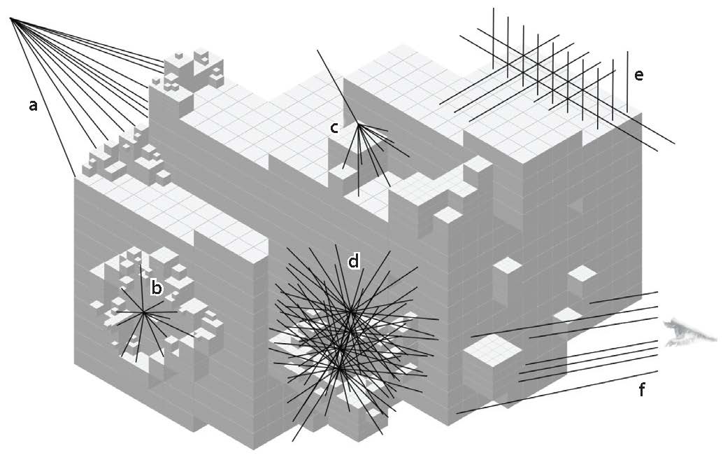Figure 3. Illustration of the various types of rays used in three-dimensional dust radiative transfer calculations performed within an adaptively refined density grid. Only a small fraction of the typical number of rays are shown for (a) an outer radiation source, (b) an inner radiation source, (c) a scattering event, (d) a region with an optical depth near 1, (e) a coarse regular outer grid, and (f) rays to the observer.

In RayT, precalculation steps are done to analyze the specific RT problem and accelerate the computations. The optical depth affects the transport within the domain, the thermalization of the radiation, and the appearance of the object on the τ(λ) ≈ 1 surface for the observer. Therefore a penetration depth analysis is performed at all wavelengths, which determines the optical depth distribution with respect to all discrete sources and the observer (see, e.g., Steinacker, Bacmann & Henning 2002). For this calculation, rays are placed from the sources to all grid cells (Figure 3a,b). In addition, we calculate the optical depth from the source to the cell using

(22)

with the ray crossing N_c cells with their individual κ_i, ρ_i, and crossing length Δs_i. τ_sou ≈ 1 marks the region where most of the source radiation is reprocessed.

The solver also calculates the optical depth from each cell to the observer τ_obs as described above (Figure 3f). This information helps us understand which regions are shielded at which wavelengths from the observer, and to calculate the final images once the main RayT has been performed.

The second precalculation is to propagate the initially deposited discrete source energy and the radiation field at the domain boundary through the domain. The calculation is done on a regular grid of rays such as that shown in Figure 3e. This calculation also determines the optical depth between cells, τ_cc, on a coarse spatial grid at all wavelengths, therefore providing information on which regions in the domain exchange significant amounts of radiation. In star formation applications, for example, regions often do not connect significantly at UV wavelengths.

If the source of radiation is the interstellar radiation field, the precalculation can be very time-consuming, as it comprises rays from all directions to all cells at all wavelengths for which the optical depth can reach 1. However, there are many cases where this precalculation is less time-consuming. For example, when the dust properties are constant in the domain, the optical depth is τ_sou = κ N_col, and this is an integral over the density only.

The main RayT calculations are performed separately for each wavelength. Rays are placed through the grid points in the τ_sou ≈ 1 layers covering all directions. In this way, additional resolution is provided where the largest changes in the radiation field are expected. Moreover, additional rays from discrete sources are placed to help resolve the illumination of the τ_sou ≈ 1 layers. This can be important, for example, in the case of an accretion disk atmosphere that is illuminated by a protostar through a narrow solid angle. The order in which the computation is done for each wavelength influences the convergence. In RayT, information has already been transported from the sources to the cells during the precalculation step. Therefore, starting with wavelengths covering the peak of the re-emitted photon energy (e.g., in the MIR) can speed up the information transport in thermally dominated problems. For problems dominated by low optical depths in the UV/optical, the order is less important as the dust self-heating is small compared to the dust heating from UV/optical photons.

In practice, the placing of rays is controlled by the maximal number of rays per cell N_l and the width of the τ_sou ≈ 1 layers: Δ τ_l, where |τ_sou − 1| < Δτ_l.The placing and iteration over wavelength is stopped when the change in the energy deposited in all cells drops below a chosen change limit and the mean field distribution has been determined. If the energy does not converge after placing N_l rays in all cells within the τ_sou ≈ 1 layers, a second run with all rays is performed, using the updated energy information from the first run. If still no convergence is obtained in this run, N_l is increased to improve the resolution. The number of rays for typical 3D dust RT applications can easily exceed 10⁶.

The final step is to calculate the radiation that is received by the observer from each cell. This calculation makes use of the precalculated τ_obs. Moreover, radiation received directly from the inner and outer discrete sources as well as from the background radiation that is inside the field of view is calculated by placing rays from the sources and the background to the observer.

To illustrate how the rays are placed in various situations, we present a few simple examples. The first is a molecular cloud core with a gas mass of 1 M_⊙ that is illuminated by a strong MIR radiation field that dominates its thermal budget. The core has no internal source of radiation except the thermally emitting dust; furthermore, the self-heating of the dust by neighboring dust grains within the core can be neglected. The precalculations will not yield any τ surfaces, given that the optical depth is too low in the MIR radiation field. The main calculation will therefore be to propagate the external anisotropic radiation field through the core with little need for refinement, by placing additional rays. Correspondingly, the rays can be placed dense enough in direction space to resolve all features of the extended illumination source (e.g., a nearby PDR; see Steinacker et al. 2005).

The second example is a binary star surrounded by a circumstellar disk. The precalculation will identify the inner disk and the disk surface as the τ ≈ 1 zone for the NIR wavelengths. The ray pattern will therefore be dense at the inner rim, and in the zone above and below the disk. At MIR or longer wavelengths, the ray pattern will be less dense in the atmosphere, given that the τ ≈ 1 range will move deeper into the disk, as the thermally emitting inner dust is important. This application has an additional complication in that it requires calculating the scattered light (see below).

A central source illuminating more complex structures is a problem for all RT solvers: A proper resolution requires many spatial cells and therefore many rays from the star to the cell and from the cell into the surrounding regions. For RayT, if a fixed direction grid is used, more and more cells are overlooked when the diverging rays reach the outer regions. For such applications, beam splitting can be used to split a ray in order to sample several neighboring cells (Abel & Wandelt 2002).

4.2.2. INCLUDING SCATTERED RADIATION    Whereas the thermal source contribution can be calculated using the mean intensity J(x, λ) per cell, the scattered light intensity depends on the direction of the incoming radiation, the optical depth for scattering, and the phase function of the grains. The RayT scheme that includes thermal reradiation and scattering must therefore store J and the intensity and direction of the incoming radiation for each cell and wavelength.

Every RayT step is expanded to include directly scattered light by calculating the amount of radiation that is scattered toward the observer using the precalculated τ_obs. In many applications, this singly scattered radiation is a good fraction of the total scattered light in the computational domain. Including multiple scattering in RayT methods significantly increases the computational requirements. Applications using 3D dust RT based on RayT with scattering sources have been presented for massive disk candidates (Steinacker et al. 2006) and grain growth in molecular cloud cores (Steinacker et al. 2010). Additional codes using RayT solvers and alternative techniques to deal with high optical depth are described in Pinte et al. (2009) and the references within. Fortunately, there are specific astrophysical regimes in which multiple scattering is not crucial or reasonable approximations can be made to limit the computational requirements.

The standard ISM dust grain distribution can be approximated as a mean grain with a 0.1 - µm grain size. Such grains have very low scattering efficiency in the MIR and, thus, scattering is often neglected if calculations are done at MIR or longer wavelengths. However, caution should be exercised, as coagulated grains in dense molecular clouds scattering can be be important even at MIR wavelengths (Steinacker et al. 2010). In addition, dust grains have a strongly forward-peaked scattering phase function, and a portion of the scattered light can be transported along the already calculated rays (see, e.g., Steinacker et al. 2003). For the wavelengths in which dust shows a more isotropic scattering phase function (e.g., MIR), additional rays can be added to carry the scattered radiation. Adding scattering is fairly straightforward in, for example, modeling star formation regions. Models of these regions will have a high number of rays in cells that are identified using the τ ≈ 1 search algorithm, allowing scattering to be calculated along existing rays. Finally, the high albedo of dust grains and the distribution of the scattered intensity over the unit sphere naturally reduce the intensity of the scattered radiation with subsequent scatterings allowing an intensity threshold to be used to limit the number of scatterings needing to be calculated.

In astrophysical objects where the optical depth is very small, or very large, or where the τ ≈ 1 layer is not resolved, calculating multiple scatterings can be ignored. If τ ≪ 1 for an object (e.g., the diffuse ISM or the zodiacal light), then single scattering completely dominates the scattered intensity, and multiple scattering can be ignored. For τ ≫ 1, the main modeling goal is usually to calculate the thermal dust emission. Because scattering is generally important at optical and shorter wavelengths, most of the energy at these wavelengths is absorbed in the τ ≈ 1 regions of the object. Thus, not calculating the scattered light properly will not have a large impact on the dust emission results. For very embedded sources such as massive young stellar objects, the stellar energy is completely converted to radiation at MIR or longer wavelengths before it leaves the core, and therefore scattering does not influence the outer radiation field. Finally, if a model does not resolve optically thick regions (e.g., in some extragalactic applications) and thus does not have τ ≈ 1 regions, then all the rays can be used to determine the global field and to transport the singly scattered radiation.

4.3. Ray-Tracing Error Analysis

Machine precision limits the precision of a solution for the RTE along a ray, through a spatial grid on which the opacity and source terms are described analytically. This can be done only with machine precision errors. For example, the previously mentioned Runge-Kutta solver with adaptive step-size control provides a good compromise between accuracy and computational cost, while providing explicit error control.

The main source of error for solutions on a single ray is the interpolation error of the density and source function from the underlying grid. It can accumulate if the density grid shows strong (and partially unresolved) gradients. The precalculation of τ ≈ 1 regions and shielded areas helps to characterize how well the chosen grid describes the underlying physical problem; refining the grid with this information can reduce the interpolation errors in the intensity distribution. Unlike solvers that calculate the intensity on a grid (e.g., finite-difference solvers), RayT solvers create no diffusive errors (i.e., beam smearing).

There is no general formula for the global error in the achieved intensity distribution, because deviations caused by coarse resolution due to the placement of rays are hard to quantify. A good test for the global accuracy of the thermal conversion of radiation is to calculate the energy output of the source term integrated over the domain, and to compare it to the energy in the radiation leaving the domain. Another test for the overall resolution of the important regions in the domain is based on the number of crossing rays per cell. All the cells that contribute significantly to the radiation field overall should be crossed by many rays. Having important cells with minimal rays is an indication that the grid was underresolved.

A practical test to understand and measure the global error is to increase the spatial or wavelength resolution by inserting more rays or adding wavelength grid points, and testing the stability of the solution.