Copyright © 2013 by Annual Reviews. All rights reserved
| Annu. Rev. Astron. Astrophys. 2013. 51:63-104
Copyright © 2013 by Annual Reviews. All rights reserved |


Until the mid-1990s, few RT codes could handle the absorption, scattering, and thermal emission by interstellar dust in general 3D geometries. The available codes were either limited to 1D or 2D geometries, or were not able to calculate the full 3D problem (e.g., missing either scattering or thermal emission). The spectacular increase in computational capabilities during the past two decades, as well as the development of more powerful techniques to solve the RT problem, has led to the creation of many 3D RT codes. To our knowledge, there are almost 30 operational codes that can handle the full dust RT problem, i.e., including absorption and multiple anisotropic scattering in a general 3D geometry. Table 1 gives a list of published 3D dust RT codes that have been or are being used for astronomical applications. The application fields of the different codes vary widely, ranging from prestellar cores and circumstellar discs to AGN and galaxies.
| Code name | Type | Reference | Main application |
| SKIRT | MC | Baes et al. (2003, 2011) | Galaxies, AGN |
| (no name) | MC | Bethell et al. (2004, 2007) | Star-forming (SF) clouds |
| TRADING | MC | Bianchi, Ferrara & Giovanardi (1996), Bianchi (2008) | Galaxies |
| RADISHE | MC | Chakrabarti et al. (2007), Chakrabarti & Whitney (2009) | Galaxies |
| (no name) | MC | Doty, Metzler & Palotti (2005) | SF clouds |
| RADMC-3D | MC | Dullemond (Manusc. in prep.) | SF disks |
| MOCASSIN | MC | Ercolano, Barlow & Storey (2005) | Photoionized regions |
| (no name) | MC | Fischer, Henning & Yorke (1994) | SF disks |
| (no name) | MC | Gonçalves, Galli & Walmsley (2004) | SF clouds |
| STOKES | MC | Goosmann & Gaskell (2007) | AGN |
| DIRTY | MC | Gordon et al. (2001), Misselt et al. (2001) | Galaxies, nebulae |
| TORUS | MC | Harries (2000), Harries et al. (2004) | SF disks |
| (no name) | MC | Heymann & Siebenmorgen (2012) | SF disks, AGNs |
| SUNRISE | MC | Jonsson (2006), Jonsson, Groves & Cox (2010) | Galaxies |
| CRT | MC | Juvela & Padoan (2003), Juvela (2005) | SF clouds |
| (no name) | MC | Lucy (1999, 2005) | supernovae |
| MCMax | MC | Min et al. (2009, 2011) | SF disks |
| STSH | MC | Murakawa et al. (2008) | SF disks |
| MCTRANSF | MC | Niccolini, Woitke & Lopez (2003), Niccolini & Alcolea (2006) | SF disks |
| mcsim mpi | MC | Ohnaka et al. (2006) | Carbon stars |
| MCFOST | MC | Pinte et al. (2006) | SF disks |
| HYPERION | MC | Robitaille (2011) | SF clouds |
| PHAETHON | MC | Stamatellos et al. (2004, 2005) | SF cores |
| STEINRAY | FD | Steinacker et al. (2003) | SF disks |
| RayT | Steinacker, Bacmann & Henning (2006) | SF cores | |
| (no name) | FD | Stenholm, Stoerzer & Wehrse (1991) | SF disks, AGNs |
| HO-CHUNK | MC | Whitney & Wolff (2002) | SF disks |
| MC3D | MC | Wolf & Henning (2000), Wolf (2003b) | SF disks, SF cores, AGNs |
| (no name) | MC | Wood & Reynolds (1999), Bjorkman & Wood (2001) | SF disks, galaxies |
| (no name) | RayT | Xilouris et al. (1997), Misiriotis et al. (2000) | Galaxies |
With many different codes and several techniques available, it might be difficult for a potential user or future developer to decide which one to choose. The choice for a given code or solution technique should be driven primarily by the specific nature of the problem being solved. Although most of the 3D codes in Table 1 are applicable for a wide range of RT problems, virtually all of them have been developed with a particular application in mind, and hence have been optimized for that particular goal.
The programming language can also influence the choice; most existing 3D RT codes have been coded in FORTRAN, C, or C++. There are no features in the 3D RT problem itself or the two solution methods presented in this review that make certain languages preferential to others. The main driver is speed: Because the 3D RT problem is computationally very challenging, all codes should be developed in a language suitable for high-performance computing. Moreover, parallelization is becoming increasingly important as a means to increase computational speed and memory availability. Several codes are designed to work on shared-memory or distributed-memory clusters and/or adopt graphical processing units (e.g., Jonsson 2006, Jonsson & Primack 2010, Baes et al. 2011, Robitaille 2011, Heymann & Siebenmorgen 2012).
The choice of a given code or method primarily depends on the specific needs of the application and/or the personal preferences of the user or developer. Nevertheless, the different approaches have some general strengths and weaknesses. These need to be considered as rough guidelines only, as there are significant differences among codes based on the same approach. For example, simple MC codes based on the naive techniques explained in Section 5.1 are many orders of magnitude less efficient than modern MC codes that use weighting schemes.
Generally speaking, setting up a reasonably efficient 3D MC RT code can be done in the time taken to do a PhD. Most MC RT codes are intrinsically 3D codes, and hence the shift from 1D or 2D codes to a full 3D geometry is fairly straightforward. For RayT codes, however, the increase in complexity when moving from 1D and 2D to 3D is much steeper. These differences explain the relative scarcity of general 3D RayT codes compared with the MC codes in Table 1; a similar comparison of 1D or 2D codes would result in a table with a much larger fraction of RayT codes. A big part of this complexity lies in the placement of the rays, which needs manual adjustment in RayT codes but is done automatically in MC codes. The RayT precalculation step needed for the manual placement of rays reveals an advantage for the MC method, as it identifies the critical locations in the model that dominate the appearance of the object. Other advantages of the MC method are that it needs less storage than RayT codes when scattering is included, and that it is widely used with many coders in the community improving its application to astrophysics with new algorithms, whereas RayT methods are mainly improved outside astrophysics. One strength of the RayT codes is the stronger and explicit error control. For example, the precalculation step can identify areas that are potentially under-resolved, allowing for changes to the grid to provide adequate resolution for the full calculation. At this point, MHD codes tend to use RayT rather than MC techniques (e.g., Heinemann et al. 2006, Kuiper et al. 2012).
Probably the most objective way to compare the strengths and weaknesses of the different codes is to use benchmark problems. In the past few years, there have been benchmark efforts in many different computational astrophysics areas, including molecular line transfer (van Zadelhoff et al. 2002), halo and void finder algorithms (Colberg et al. 2008, Knebe et al. 2011), astrophysical hydrodynamics (Agertz et al. 2007), cosmological hydrodynamical simulations (Frenk et al. 1999, O'Shea et al. 2005), and cosmological radiation hydrodynamics (Iliev et al. 2006, Iliev et al. 2009). At the moment, no code validation or benchmark project exists for 3D dust RT. The most advanced dust RT code validation projects are 2D benchmarking efforts.
Pascucci et al. (2004) presented a benchmark test for 2D equilibrium RT problems. Their system consists of a single star surrounded by a flared axisymmetric accretion disc. The optical depth through the disc varies from τV = 0.1 to τV = 100. The accretion disc contains strong density gradients, which makes it an ambitious benchmark problem (unfortunately, anisotropic scattering is not taken into account). The authors compare the temperature maps and SEDs for five 2D dust RT codes (two grid-based codes and three MC codes). Differences between the various codes in the temperature maps are smaller than 1% for the most optically thin model, but some reach up to 15% in the most optically thick system. For the emerging spectra, the differences range from a few percent for the optically thin models to more than 20% for the most optically thick models.
A first extension of the Pascucci et al. (2004) benchmark test was presented by Pascucci et al. (2003), with two of the five codes from the original benchmark participating (one MC code and one RayT code, both intrinsically 3D codes). [The Pascucci et al. 2003 paper was actually a follow-up project.] They considered a similar disc as that in the Pascucci et al. (2004) benchmark, with an azimuthal ring added as a simplified model for a spiral density distortion. The main advancements were the addition of anisotropic scattering and that images and visibilities, in addition to SEDs and temperature maps, were compared. The difference in flux in the entire image was smaller than 20%, but the visibility curves showed substantially larger discrepancies in their overall shapes.
Pinte et al. (2009) go another step further in what is the most advanced dust RT benchmark to date.They start from a similar circumstellar disc model, but consider optical depths up to τV =106, use anisotropic scattering, and compare images and polarization maps. The four different codes that participate in the benchmark are all MC codes. The agreement in the temperature distributions is very good, with differences almost always smaller than 10%. Differences in the SEDs remain smaller than 15% for models with τV =1,000 and agree within 20% over almost the entire wavelength range for the most optically thick cases. Pixel-to-pixel differences in high-resolution scattered light images remain limited to 10%, and the polarization maps do not differ by more than 5° in regions where the polarization can be effectively measured by observations (Figure 7).
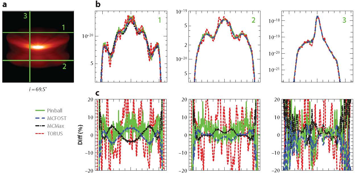 |
Figure 7. An example of the two-dimensional dust radiative transfer benchmark (Pinte et al. 2009) for a flared circumstellar disc with a V-band optical depth in the midplane of τ = 106. (a) Scattered light image. (b) These three panels show brightness profiles along the cuts plotted in panel a. (c) The differences among the four different models used in the benchmark. The different line styles and colors indicate whether the model was Pinball (Watson & Henney 2001), MCFOST (Pinte et al. 2006), MCMax (Min et al. 2009), or TORUS (Harries et al. 2004). |