Copyright © 2013 by Annual Reviews. All rights reserved
| Annu. Rev. Astron. Astrophys. 2013. 51:63-104
Copyright © 2013 by Annual Reviews. All rights reserved |


The uses of 3D dust RT codes are many. They range from helping us understand the impact of locally clumpy dust on dust RT (Witt & Gordon 1996, 2000, Bianchi 2008), to modeling observed images of objects to derive the source and dust distributions (De Looze et al. 2012b, Gordon et al. 1994, Steinacker et al. 2005), to predicting the appearance of an object that has been modeled with an HD code (Steinacker et al. 2004, Bethell et al. 2004, Jonsson, Groves & Cox 2010, Robitaille 2011), to investigating the ensemble behavior of objects to derive average source and dust properties (Law, Gordon & Misselt 2011), and to testing observability of objects for instrument and observation planning (Wolf 2008, Gonzalez et al. 2012). To illustrate the challenges in modeling observations, we focus on the modeling of objects to derive their physical properties from observational data. The common approach is to perform some steps of the following scheme:
Although the scheme seems straightforward, the full set of steps has rarely been carried out for existing, published 3D dust RT models, as each of these steps provides challenges for 3D dust RT.
The aim is to choose an appropriate model that allows meaningful physical information to be derived from the given observational data. This is a general topic, but 3D RT modeling has special features that are important to consider. The data are usually SEDs and/or images, and we can investigate the number of independent information bits a priori, for example, by counting the number of wavelengths for which the flux density values have been measured. This is then compared to the number of model parameters.
Most 3D models include 10 to several hundreds of free parameters, depending on the complexity of the spatial model and the assumed dust properties. Even for attempting to reproduce only the global SED of an object, it is difficult to stay below 10 parameters, given that modeling a dusty 3D structure requires a few length scales and/or power laws to describe the density, dust properties, and viewing angles. Figure 5 illustrates the large number of free parameters needed to reproduce the 3D dust distribution of a molecular cloud. Figure 6 shows four examples of state-of-the-art RT fits to dusty galaxy images. Such RT model fits are designed to determine the parameters that describe the intrinsic 3D distribution of stars and dust in both large-scale geometric parameters (e.g., stellar and dust scale lengths and heights) and measures of the small-scale inhomogenity or clumpiness of the dust.
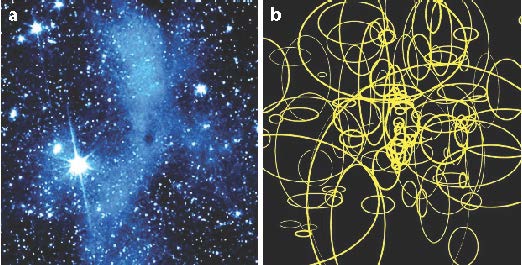 |
Figure 5. (a) Spitzer Space Telescope image of the molecular cloud L183 at 3.6 µm revealing "coreshine", which is scattered light from the densest part of the cloud. (b) Spatial modeling based on basis functions that have Gaussian density structures in all three coordinates (Steinacker et al. 2010). The ellipses give the full width at half maximum of the various Gaussians in the plane of sky. |
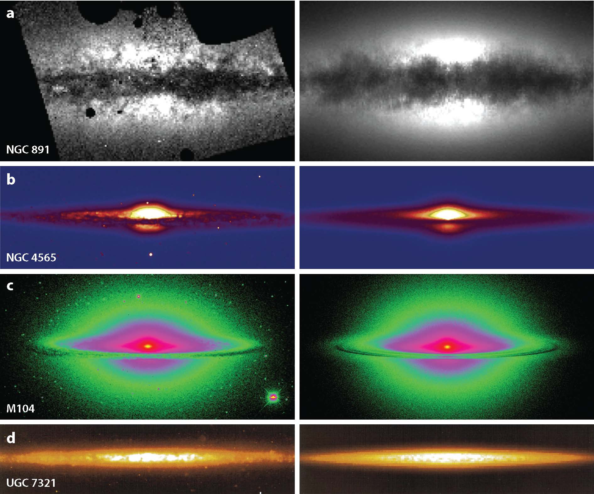 |
Figure 6. Examples illustrating the current state of the art in fitting dust radiative transfer models to images of galaxies. The left panels show the observed images; the corresponding panels on the right are the fits to these images. (a) A clumpy three-dimensional (3D) spiral galaxy model fit to a Hubble Space Telescope B-band image of the prototypical edge-on spiral galaxy NGC 891 (Schechtman-Rook, Bershady & Wood 2012). (b) A 2D disc galaxy model fit to a Sloan Digital Sky Survey g-band image of NGC 4565 (De Looze et al. 2012a) using a fully automatic fitting based on genetic algorithms (De Geyter et al. 2013). (c) A detailed 2D model for the Sombrero galaxy, fit to a V-band image (De Looze et al. 2012b). (d) A 3D clumpy disc model fit to an R-band image of the edge-on low surface brightness galaxy UGC 7321 (Matthews & Wood 2001). |
Starting with more free model parameters than data points is often considered to produce meaningless parameter values. However, a careful exploration of the parameter space can detect ambiguities and reveal redundant parameters. As long as the parameter space exploration can be afforded computationally, starting with a detailed model and analyzing the parameter ambiguities is usually the most accurate way to model an object.
As discussed in Section 3, there are a variety of options for discretizing space, direction, wavelength, and the dust model. If the grid fails to resolve structures that are important at a particular wavelength, the corresponding model image will be inaccurate. A good example is the surface layer of an accretion disk illuminated by a central star. If the layer is not resolved well, the description of the radiation field that is scattered in the layer will be poor and the scattered light images inaccurate. Therefore, the discretization step often includes running the RT code before the start of the modeling to verify that expected features are present in the image or SED and that changes/refinement do not influence the overall appearance of the object.
6.3. Comparison of Models and Data
Once the model images or SEDs have been calculated, the results should be convolved with the beam of the observed instruments/telescopes, and the sampling should be made equal (pixel size for images). It is important to apply detection limits, especially when studying faint structures. For interferometric observations, the incomplete coverage of all spatial scales implies that the comparison should be performed in the (u,v) plane rather than the spatial plane to achieve the highest fidelity. Calibration uncertainties and correlated noise properties in the observations should be understood and included in the model, as opposed to observations comparison alone. In addition, foreground emission (e.g., caused by the zodiacal light) should be carefully removed or modeled, especially for on-off chopping observing modes that remove this emission as part of the data reduction process. Generally, modelers can benefit from good communication with experienced observers. Another potential source of error in comparing model results and data can be a displacement of structures due to observational uncertainties. Additional translation parameters can correct this and provide physical insight by deriving improved positioning.
6.4. Exploration of the Parameter Space
The parameter space of 3D dust distributions is large: A uniform coverage of a 10D parameter space with five grid points in each parameter, would imply ~ 10 million individual RT calculations. Therefore, almost all 3D RT modeling of data has been done "by hand", that is, starting from a point in the parameter space and then varying just one parameter to explore the variations in the results. This drastically reduces the coverage in parameter space at the expense of exploring correlations between parameters. In structures with strong gradients, inhomogeneously distributed radiation sources or varying optical depth, the resulting radiation field may react strongly to changes in the model parameter. In this case, low-coverage by hand explorations are likely quite unreliable.
To evaluate the model and the variation in the model parameters, the difference between the model data and the observed data must be defined (often using a χ2 metric), and the fitting procedure must then be to minimize this difference by varying the parameters. Some standard optimization methods applied in astrophysics are gradient descent, Newton's method, Metropolis optimization, and genetic algorithms. The latter two are able to leave local minima with the goal of ending in the deepest minimum providing the best-fitting model parameters.
There are advancements in the application of automated fitting techniques that are already in use for 2D RT calculations and are starting to be used for 3D RT calculations as well. One such technique is the Metropolis algorithm that has been applied to 3D dust RT in the form of simulated annealing (Steinacker et al. 2005). Precomputing a large grid of models is a promising technique. Robitaille et al. (2007) used a parametrized circumstellar disk model to create a large grid of precalculated SEDs for a 2D configuration and then used the grid to fit the disk parameters and to characterize uncertainties in fit parameters. Other promising techniques are 2D RT fitting techniques based on the Levenberg-Marquardt algorithm (see, e.g., Xilouris et al. 1999), the downhill-simplex method (Bianchi 2007), and genetic algorithms (De Geyter et al. 2013). Some of these techniques have already been applied to 3D structures, albeit in limited parameter spaces (see, e.g., Witt & Gordon 2000; Schechtman-Rook, Bershady & Wood 2012).
Quantifying the ambiguity of the derived parameters is also important. The 2D circumstellar disk modeling of SEDs in Robitaille et al. (2007) provides a template for determining the ambiguity when a complex model is applied to only a few SED points. A general strategy to assess ambiguity is to explore the variation of the fitting metric (e.g., χ2) in the vicinity of the best-fit parameters and characterize the overall degree of variation by random or grid-based parameter space exploration.
Each of the RT solvers has its own sources of errors due to approximations, the underlying grid, undetected regions of the computational domains, etc. Tracing these errors, measuring them, and estimating their importance is nontrivial. RayT provides error control for the solution along one ray, and MC can provide error control on the number of photons needed; however, whether the rays are sent through the right parts of the domain is not well quantified. For modeling, a comparison of these errors with the solution and observational errors determines the sensitivity of the observed data to the specific science question of interest.
The true challenge of RT modeling is to invert it, i.e., determine the 3D density structure of the dust and the sources, and the dust properties from a set of images taken at different wavelengths. Direct inversion is computationally impossible in 3D with current or expected computing capabilities. In 1D, an analytic inversion can be performed under special assumptions (Steinacker, Michel & Bacmann 2002), and numerical 1D inverse RT modeling was used in Doty et al. (2010). A forward RT method using many iterations provides a good solution but is limited to fairly simple RT applications. A prominent difficulty is the loss of information due to the line-of-sight integration inherent in the observations. Multiwavelength observations can help disentangle the line-of-sight integration. For example, points in the center of a molecular core are better shielded and cold compared with points in the outer parts, so millimeter observations can be used to constrain the core center and shorter wavelength observations to constrain the outer parts. Such molecular cores are simple enough to enable inverse RT to be done. For example, Steinacker et al. (2005) used a 3D background radiation field illuminating a 3D model core and fitted the MIR and millimeter images of the core ρ Oph D, deriving the density and temperature structure with assumed dust properties.