


The rotation curves (RCs) of spirals are an accurate proxy of their gravitational potential. We measure recessional velocities by Doppler shifts, and from these (often 2D) data, we construct the RC V(R). This process estimates also the sky coordinates of the galaxy kinematical center, its systemic velocity, the degree of symmetry and, often, the inclination angle.
Notice that the effectiveness of the RC is proved in many ways: e.g., in systems with MI < −18 in the innermost luminous matter dominated regions the gravitating mass (measured by V(R)) agrees with the predictions from the light distribution (Ratnam and Salucci 2000).
The rotation curves in disk systems have 3 different components: the relationship with the total gravitational potentials φtot = φb + φH + φdisk + φHI is
 |
(13) |
Then, the velocity fields Vi are the solutions of the four separated equations: ∇2Φi = 4 π G ρi where ρi are dark matter, stellar disk, stellar bulge, HI disk surface/volume densities (ρh(r), ρbu(r), µd(r) δ (z), µHI(r) δ (z) with δ(z) the Kronecker function, z the cylindrical coordinate) and φi the gravitational potential.
Recently, a new way to exploit the RC to obtain the DM halo density distribution has been devised (Salucci et al. 2010). We assume that spirals are composed by a stellar disk (Freeman 1970), a HI disk and an unspecified spherical DM halo with density profile ρH(r). Other baryonic components can be added, if needed. 3 From the radial derivative of the equation of centrifugal equilibrium we obtain
 |
(14) |
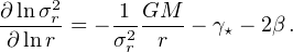
We have aD(r) = [GMD r / RD3] (I0 K0 − I1 K1), where In and Kn are the modified Bessel functions computed at r / 2 RD. Noticeably, the second term of the r.h.s. of Eq. (14) goes exponentially to zero for r / RD > 2 (see Fig. 5). Then, for R > 2 RD, we can determine the DM density profile (see Fig. 5). On the other hand, for R < RD, the DM distribution is negligible, so that, if we have a good spatial coverage of the inner RC, we can use Eq. (14) also to obtain the disk mass with good precision.
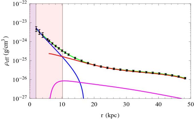 |
Figure 5. A test case: NGC 3198. Effective total density (points with errorbars). Contributions: stellar disk (blu), HI disk (magenta), dark matter (green line), all components (green). Regions in which the method: 1) is not applicable (pink), 2) provides us with a) the value of disk mass (green) b) the halo density profile (white). Image reproduced with permission from Karukes et al. (2015), copyright by ESO. |
4.2. A reference velocity for disk systems
In spite of the fact that V(R), the circular velocity, is a function of radius we often require a meaningful reference velocity to tag each disk system. In the literature there is no shortage of proposed reference velocities, among those: Vflat, Vlast, the linewidths W20, W50 and the maximum velocity Vmax. Obviously, if the RC of an object is not available, we are forced to choose one of these kinematical measurements as a reference velocity, however, we must stress that they are very biased: a) a flat part of the RC occurs only a limited number of objects and only over a limited radial region (Persic, Salucci and Stel 1996); b) Vlast depends on the distribution of HI in the galaxies and on the sensitivity of radio telescope used; c) the linewidths are similar to the case b) and furthermore they depend on the full RC profiles; d) the significance of Vmax changes as galaxy luminosity changes, sometimes coinciding with the outermost available velocity, in other cases, with the innermost one. The best unbiased reference velocity for spirals is the quantity: V(k RD) that also involves the stellar disks length scale. We have k = 2.2 or 3.2, according whether we are investigating the properties of the luminous or of the dark matter.
The main goal of the DiskMass Survey (Bershady et al. 2010a, 2010b) was to determine the dynamical mass-to-light ratio of the galaxy disks (M / L)dyn by a suitable use of the stellar and gas kinematics. At a radius R, for a locally isothermal disk, we have
 |
(15) |
where the value b = 1.5 is a reasonable approximation for the composite (gas+stars) density distribution (van der Kruit 1988), I the surface luminosity obtained from the photometry, σz the vertical component of the stellar velocity dispersion. Noticeably, with the advent of 2-dimensional spectroscopy using integral field units (IFU), the accuracy and the z-extension of the measurements of σz has been dramatically increased; hz is the disk scale height (van der Kruit and Searle 1981, Bahcall 1984) that can be directly measured, and that well correlates with the disk scale length RD (Kregel et al. 2002, Bershady et al. 2010a).
Let us stress that this approach leading to Eq. (15) is certainly a new avenue for investigating dark matter in galaxies, but some warning must be raised in that it can be subject to relevant biases (Hessman 2017).
It is well known that in spheroids the kinematics is complex, the stars are in gravitational equilibrium by balancing the gravitational potential, they are subject to, with the pressure arisen from the r.m.s. of their 3D motions. Moreover, we cannot directly measure the radial/tangential velocity dispersions linked to the mass profile, but only their projected values (e.g., Coccato et al. 2009).
The SAURON (Bacon et al. 2001) Integral Field Spectroscopy survey (de Zeeuw et al. 2002) was the first project to map the two-dimensional stellar kinematics of a sample of 48 nearby ellipticals with MB < 18. This survey was followed by the ATLAS3D project (Cappellari et al. 2011), a multiwavelength survey of 260 ETGs galaxies. In Cappellari (2016) one finds the details of these observations.
The dispersion velocity is related to the gravitational potential of a galaxy by the Jeans equation that we express as (Binney and Tremaine 2008)
 |
(16) |
Here, G is the gravitational constant and M(r) is the enclosed mass. The velocity anisotropy β = 1 − σθ2 + σφ2 / 2 σr2, where σθ, φ, r are the velocity dispersions in the r, θ and φ directions, can be a function of radius r (Binney and Tremaine 2008). It is useful to define: α = d logσr / d logr. Almost always the motions in the θ and φ directions are assumed to coincide.
ν⋆ is the 3D stellar density distribution, γ⋆ = d logν⋆ / d logr. Under the assumption of constant β, the radial velocity dispersion σr(r) can be expressed as
 |
(17) |
We can then determine the galaxy mass profile by means of Eq. (17) and the line-of-sight velocity dispersion σl.o.s. when the anisotropy factor β(r) is known or assumed:
 |
(18) |
where I(R) and ν⋆(r) are related by I(R) = 2 ∫r+∞ [ν⋆(r) r dr / √r2 − R2]. I(R) and σl.o.s.(R) are directly measured.
The Schwarzschild method can be seen as a (complex) extension of the Jeans method and it is especially applied to dSph galaxies where the stellar component is totally negligible (Cretton et al. 1999, Breddels et al. 2013). It is based, fixed a specific gravitational potential, on the integration of test particle orbits drawn from a grid of integrals of motions, i.e., the energy and the angular momentum. The main feature of this method is that, differently from the Jeans method, it can successfully use the observed second and fourth velocity moment profiles to break the mass-anisotropy degeneracy (Breddels et al. 2013).
In the case of objects (e.g., S0 galaxies) in which the dispersion velocity combine with the rotation motions to balance the galaxy self-gravity, there is a simple and efficient anisotropic generalization of the axisymmetric Jeans formalism which is used to model the stellar kinematics of galaxies (see Cappellari 2016 for details). The following is assumed: (i) a constant mass-to-light ratio M / L and (ii) a velocity ellipsoid that is aligned with cylindrical coordinates (R,z) and characterized by the classic anisotropy parameter βz = 1 − σz2 / σr2. These simple models are fit to integral-field observations of the stellar kinematics of fast-rotator early-type galaxies. With only two free parameters (βz and the inclination) the models generally provide remarkably good descriptions of the shape of the first (V) and second (Vrms ≡ √V2 + σ2) velocity moments. The technique can be used to determine the dynamical mass-to-light ratios and angular momenta of early-type fast-rotators and it allows for the inclusion of dark matter, supermassive central black holes, spatially varying anisotropy, and multiple kinematic components.
4.6. Dispersion velocities versus rotation curves
Here, it is worth making a comparison between the circular velocity V(r) and the radial (or line-of-sight) velocity dispersion of an irrotational gravitational tracer with distribution ν⋆(r) and with anisotropy β(r). From Eq. (16) we get:
 |
(19) |
α(r) and γ⋆(r) are the logarithmic derivatives of σl.o.s. and ν⋆. Let us notice that, in dispersion velocity supported systems, even in the case of isotropic orbits: β(r) = 0, it is necessary to know the spatial distribution of the tracers in order to make any inference on the DM distribution. Flat RC and flat dispersion velocity profiles do not necessarily indicate the same gravitational field.
4.7. Masses in spheroids within half-light radii
We can measure the total mass enclosed within the half-light radius R1/2 by measuring σl.o.s.(R1/2) the line of sight velocity dispersion at this radius (Wolf et al. 2010). Since σtot2 = σr2 + σθ2 + σφ2 = (3 − 2 β)σr2 we can write the Jeans equation as G M(r) r−1 = σtot2(r) + σr2(r) (−γ⋆ + α −3 ). Let us define R3 as γ⋆(R3) = 3 4 since α(R3) ≪ 3 from the observed σlos(r) profiles, then, at R = R3, we have, independently of the value of the anisotropy:
 |
(20) |
APOSTLE cosmological hydro dynamical simulations have tested the validity and accuracy of this mass estimator and found that the resulting measurements are, at most, biased by 20% (Campbell et al. 2017).
Given a number of N of tracers in dynamical pressure supported equilibrium with no systematic rotation and moving with l.o.s. velocities within a dark halo of mass profile M(r), the TME is expressed as
 |
(21) |
The prefactor C depends on i) the slope є of the gravitational potential, assumed to be: Φ(r) ∝ v02 / є (a / r)є; v02 log(a / r ) (є = 0). ii) the “slope” γ⋆ of the de-projected density profile of the tracers (ρtrac(r)∝ r−γ⋆) iii) the orbital anisotropy β of the tracers.
We then have C = [(є + γ⋆−2β) / Iє,β] rout1−є with rout the distance of the outermost tracer and Iє,β = π1/2Γ(є / (2 + 1)) / 4Γ((є / (2+ 5 )) / 2) [є + 3 − β(є + 2)], where Γ is the Gamma function (Watkins et al. 2010, An and Evans 2011).
The mass estimator in Eq. (21) performs very well, especially in the case in which the tracers are in random orbits, so that β = 0 and for ellipticals where we have α = 0 ± 0.1. In these cases, the uncertainties on the two latter quantities do not bias the mass estimate.
We briefly recall here that weak gravitational lensing is a powerful tool for probing the dark matter distribution in galaxies (Schneider 1996, Hoekstra and Jain 2008, Munshi et al. 2008, Bartelmann and Maturi 2016). It is known that observed images of distant galaxies are coherently deformed by weak lensing effects caused by foreground matter distributions. These distortions enable the measurement of the mean mass profiles of foreground lensing galaxy through the stacking of the background shear fields (Zu and Mandelbaum 2015). To determine halo mass, we measure the excess surface mass density ΔΣ(R) = Σ(< R) − Σ(R), which is the difference between the projected average surface mass within a circle of radius R and the surface density at that radius. The tangential shear γt is directly related to the above quantities through ΔΣ(R) = Σcrit ⟨γt(R)⟩, where Σc is the critical surface density defining the Einstein radius of the lens
 |
(22) |
where Ds, Dl, and Dls are the distances to the source, to the lens and the lens-source one, respectively. The lens equation relates γt with the distribution of matter in the lensing galaxy:
 |
(23) |
where Σ(R) = 2 ∫0∞ ρ(R, z) dz is the projected mass density of the object distorting the galaxy image, at projected radius R and Σ(R) = 2 / R2 ∫0R x Σ(x) dx is the mean projected mass density interior to the radius R.
Gravitational lensing occurring in very aligned galaxy-galaxy-observer structures magnifies and distorts the images of a distant galaxy providing us with relevant information on the mass structure of the intervening galaxy so as of the background source (see Treu 2010).
The lens system is axially symmetric, the radial coordinate r is related to cylindrical polar coordinates by r = √ξ2 + z2 where ξ is the impact parameter measured from the center of the lens. The mean surface density inside the radius ξ is
 |
(24) |
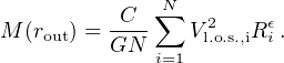
The presence of an Einstein ring of radius Re, at projected galactocentric distance ξ (see Fig. 6), allows us to obtain the projected total mass inside ξ:
 |
(25) |
 |
Figure 6. Einstein ring (artist's concept). This extraordinary GR effect provides us with the value of the projected mass of the galaxy lens inside Re. |
4.11. X-ray emission & hydrostatic equilibrium
Isolated ellipticals have an X-ray emitting halo of regular morphology, that, extends out to very large radii. The gravitating mass inside a radius r, M(r) can be derived from their X-ray flux if the emitting gas is in hydrostatic equilibrium. From its density and the temperature profiles we obtain the total mass profile (Fabricant et al. 1984, Ettori and Fabian 2006:
 |
(26) |
where Tg is the (measured) ionised gas temperature, ρg the gas density, k is the Boltzmann's constant, µ = 0.62 is the mean molecular weight and mp is the mass of the proton.
3 The HI component is obtained directly from observations, however, it is always negligible because dVHI2 / dr ≃ 0. Back.