


Now we come to the heart of the problem with Hubble's interpretation, but more importantly to the watershed for practical cosmology itself in a fundamental development that changed the field.
Reading most of the many papers on observational cosmology before the early 1960s, nowhere does one see the modern approach of solving the Friedmann equation that describes the development of the scale factor R(t) with time, and how the closed form of R(t) for arbitrarily high z is to be used to obtain the exact equations necessary to interpret the observations, valid for all redshifts. What in fact is the correct equation for the interval "distance," r, as a function of redshift?
Before the correct equations became known in the late 1950s, all relations involving observed magnitudes, angular diameters, redshifts, spatial volumes, and the consequently N(m) counts were given in Taylor series expansions in z, using only R(t0) and the first several derivatives of R(t) about the present epoch. The only assumption on R(t) was that it is a smooth enough function for the Taylor expansion to mean something. These series expansions, while good for small redshifts, were worthless for redshifts larger than perhaps 0.3, which was in fact near the limit of redshifts known even in the late 1950s.
What is remarkable about this situation is that the Friedmann equation and its solution never entered most of these papers at the interface between theory and observation. Examples are the marvelously complicated series-expansion papers by Davidson (1959a, b, 1960), and even more remarkably, the first edition of the famous text book by McVittie (1956).
The developments that began the modern era were the derivations of all the relevant equations using the Friedmann equation to give the explicit solutions of R(t) for all t (i.e., for arbitrarily high redshifts). Remarkably, the complete development is set out in two short papers by Mattig (1958, 1959).
In the first he derives the famous r(z,q0) relation
| (4.1) |
The paper is only three pages long. The second, in which he derives the volume elements (both Euclidean and noneuclidean) also as functions of z and q0 is done in only two pages. (3)
Yet these two papers changed the subject. An example is the second edition of McVittie's (1965) text book where every equation in practical cosmology is based on Mattig, in contrast to the 1956 first edition where everything is in series expansions of R(t), sans even the Friedmann equation as a guide.
The important point for our purposes is the comparison of Mattig's exact theory with Hubble's intuitive assumption for the relation between interval "distance" (4) and redshift.
Hubble's assumption for an (R0r, z) relation was,

| (4.2) |
The correct (Mattig 1958) equation for any q0 and z is equation (4.1) above, for which the two most interesting special cases are for q0 = 0 in a zero density (massless) universe, and q0 = 1/2 for flat space-time curvature. The relevant equations are
| (4.3) |
for q0 = 0, and
| (4.4) |
for q0 = 1/2, both of which differ from Hubble's assumption in equation (4.2) except near the z = 0 limit where all equations have the same z dependence. Figure 4 shows the differences between equations (4.2), (4.3), and (4.4) for progressively larger redshifts. These differences translate into different predictions of how the proper volume elements vary with redshift in geometries of arbitrary curvature.

|
Figure 4. Comparison of Hubble's assumption (upper straight line) of how the parameter "distance" that is needed in the correct cosmological equations relating volume to redshift differs from the correct "distance" -redshift relations for two values of the deceleration parameter, as calculated from the Mattig (1958) equation for r(z, q0). |
The step beyond equation (4.1) in Mattig's derivation is to use the Robertson (1938) equation for how the received flux of a source of absolute luminosity, L, varies with redshift. This equation relates the redshift and the received bolometric luminosity, l, with L and with the interval "distance" R0r from equation (4.1) as
| (4.5) |
to finally obtain the predicted count-brightness N(m) relation for galaxies distributed uniformly in Back.space. (5) This prediction also differs from Hubble's assumption that log N(m) ~ 0.6m for a space with zero curvature.
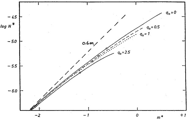
Fig. 5 shows the Mattig (1959) predictions for the N(m) count distribution in the ideal case of a single fixed absolute luminosity (a delta function luminosity distribution) for the counted galaxies, bolometric magnitudes (i.e., corrected for K dimming, both selective and non-selective), and no evolution, either luminosity or density, in the look-back time. The differences between the Hubble assumption (the upper dashed line) and the exact Mattig predictions of equations (4.3) and (4.4) above are evident in Fig. 5.
|
Figure 5. Comparison of Hubble's assumption of the expected log N(m) ~ 0.6m relation (upper dashed line) with the correct Mattig (1959) prediction (no evolution) in closed form, based on the solution of the Friedman equation, rather than on previous formulations via series expansions in z. Diagram from Mattig (1959) with Hubble's assumption put in as the dashed line. |
In this and the previous section we have seen how (1) errors in the K term evaluation, (2) errors in the apparent magnitude scale, and (3) errors in the precepts of the proper equations for "distances" and the consequent variation of apparent magnitude with distance for arbitrarily high redshifts affected Hubble's conclusions. The two remaining considerations concerning these conclusions are (a) a comparison of Hubble's N(m) count data with the modern counts, and (b) replacing Hubble's analysis that used mean values for absolute magnitude and the apparent magnitudes at given redshifts by proper distribution functions of (m, z) and (M, morphological type) luminosity functions. Consider first the modern counts.
3 In a later paper
Mattig (1968)
introduced closed equations valid for a finite cosmological constant.
Back.
4 See
McVittie (1974)
for an interesting discussion of why "distance" is an ambiguous
concept in cosmology, differing depending on the parameters used to
measure it. Because of this
ambiguity, it is necessary that no equations that connect observables
should contain "distance"
in their final form. The equations must all be constituted to contain
only the directly observed
parameters of flux, angular size, and redshift
(Sandage 1988).
Back.
5 The crucial Robertson equation (4.5)
was in contention for many years, with arguments
of various subtleties occurring between such giants as de Sitter, von
Laue, Tolman, Vogt, and
others as to whether the factors of (1 + z) in the denominator should be
as shown or rather only
the first power, or even to the third power. Robertson gave the
definitive proof of equation (4.5) in the cited reference.
Back.