


5.1. The post Hubble era (1970-1997)
The last major program begun by Hubble three years before his death was a comprehensive plan to repeat his 1934-1936 N(m) campaign using the newly completed 48-inch Palomar Schmidt telescope, commissioned in September 1948. The wide field and superb imaging quality of this miracle telescope offered substantial advantages over the coma-affected and small area photographic plates used in the 1934-1936 work.
The first plates for Hubble's newly planned galaxy count survey were taken in the spring of 1949, before the systematic Palomar Sky Survey was begun. To assist in the work, I had been sent up as a graduate student by Greenstein to the Mount Wilson office from Cal Tech. I can only now suppose that Greenstein's selection from among other graduate students in the newly created (1948) Cal Tech department of astronomy, was based on my previous experience in survey photography, star counting, magnitude transferal from Selected Areas by photographic means, and obtaining magnitude distribution functions of the counts in areas of similar absorption, gained in a junior-senior undergraduate thesis program at the University of Illinois in the Perseus and Taurus dark cloud regions of the Milky Way. (An analysis was later published by another who had no relation to the work).
The technique to be employed for Hubble's new galaxy-count program was again to count to successively fainter magnitudes on a series of plates of graded exposure times with later calibration of the various limiting magnitudes by determining the relation of the plate limits for stars and for galaxies - identical to the procedures in 1934-1936, but with a modern stellar magnitude scale in Selected Area 57 as the standard sequence.
The project was not completed for two principal reasons: (1) The conviction arose that a definitive new study must be based on the measurement of individual magnitudes for each galaxy rather than by simply counting to a plate limit. The technical means via areal photometry to do this were not in hand in the 1950s. (2) The solution to the problem of aperture corrections via growth curves to obtain either a "total" magnitude or a correction to obtain it had not then been solved (Humason et al. 1956, Appendix A). (Adequate standard profile templates had not been measured in the early 1950s). Therefore, Hubble's new count program was never begun in earnest after his death in 1953.
It was only 30 years later, beginning in the late 1970s that the modern photometric methods of individual galaxy photometry was made possible by the two-dimensional detectors and computer technology. A summary of several of the many galaxy count programs using these modern methods, completing Hubble's 1950 hopes, is the subject of this section.
The state of the count-magnitude relation just at the end of the 1930-1975 exploratory period is shown in Fig. 6 (Sandage, Tammann, Hardy 1972), combining Hubble's faint data with those of Mayall (1934), the bright counts of Zwicky to B ~ 15.7, and the vast, wide area, counts of Shane and Wirtanen (see Shane 1975), but again counting to a plate limit.

|
Figure 6. Summary of the N(m) count
distribution as the data existed in 1972, before the
major modern observational campaigns had begun. Diagram for
Sandage, Tammann,
and Hardy (1972).
See this reference for a discussion of (1) the North Galactic
Anomaly shown as the
discontinuity at bright magnitudes, and (2) the meaning of the
|
One of the first papers in the post-exploratory era (individual magnitudes determined and account taken of total vs. isophotal magnitudes) was that of Tyson and Jarvis (1979), shown in Fig. 7. They combined their data with many previous surveys to give a comprehensive summary reaching J(Gunn) = 24. The deviation of log N(J) from a slope of 0.6 is clearly seen beginning near J = 17, similar to that shown in Fig. 6 and initially discovered by Hubble (Fig. 1). An interesting point from Fig. 7 is that the surface density of galaxies exceeds that of stars for J > 22.

|
Figure 7. An early summary of the major count campaigns extending to the faint J magnitudes of J = 24. The departure of the slope from 0.6 beginning at J = 17 is consistent with the early theoretical curve fitted to the data in Fig. 6. Diagram from Tyson and Jarvis (1979). |
Fig. 8 shows the state of the work nearly a decade later, taken from a summary by Ellis (1987). The two principal features of this diagram are (a) the comparison of individual data points from various surveys, shown to illustrate the general accuracy of the count data at better than 0.2 dex in log N(m), and (b) the comparison of the data with the predicted counts from the Mattig formulation using proper distribution functions for (m, z), for the luminosity function (M, T), for K(z, sed), and for an assumption of the morphological mix of field galaxies (see next section). The excess of the counts relative to the predicted no-evolution Mattig curve is evident. It was discovered by Kron (1980) and is a feature of all subsequent surveys, forming a major subject of this workshop.

|
Figure 8. Summary by Ellis showing not only the range of differences in the counts from different modern group campaigns, but also the beginning of the now well known large excess of the counts fainter than BJ = 20, discovered by Kron (1980), relative to the predicted no evolution "standard" Mattig model. The BJ magnitudes are related to the standard Johnson B by J = B-0.1. Diagram from Ellis (1987). |
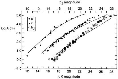
However, the degree of the excess is a function of wavelength, also discovered by Kron (1980) from his progressive blueing of the color distribution fainter than bj = 22. A summary of counts in the three band passes of bj, r, and K is in Fig. 9 from the review by Koo and Kron (1992). The important point is that the counts in K show no excess relative to the predicted N(m), whereas the counts in bj have the pronounced excess.
|
Figure 9. Summary of differential counts in bJ, r, and K reviewed by Koo and Kron (1992). A(m) is the number of galaxies per square degree per magnitude interval in the magnitude interval from m 1/2. The predicted Mattig theoretical non-evolution curves are shown for comparison. |
A particularly clear representation of the large excess at the faintest levels is in Fig. 10 from Lilly, Cowie, and Gardner (1991) in the blue pass band. Again, the predicted N(m) no-evolution relations, calculated with all the complications summarized in section 6, are shown as the dotted curves for two values of the curvature parameter.

|
Figure 10. Summary of the very deep differential [i.e., A(m)] counts showing again the strong excess of the faint counts over the no-evolution predictions for two Mattig models. Diagram from Lilly, Cowie, & Gardner (1991). |
A similar summary in B and K is given by Ellis in this volume. His diagram is reproduced as Fig. 11 here, but with the O.6m line, as in Hubble's pre-Mattig assumption, drawn, showing that the counts, even in B, are less numerous than the 0.6 relation, as indeed first discovered by Hubble in 1936. Nevertheless, the counts are larger than the theoretical no-evolution predictions, especially in B.

|
Figure 11. Count data from Ellis (this volume) but with the 0.6m line drawn to emphasize, that despite the excess relative to the no-evolution Mattig predicted N(m), the counts are still less numerous than Hubble's pre-Mattig assumption that log N(m) ~ 0.6m. |
 = 1.7 line as a prediction of a
hypothetical hierarchical distribution in depth.
= 1.7 line as a prediction of a
hypothetical hierarchical distribution in depth.