6. THE STEPS NEEDED TO MAKE A PROPER CALCULATION OF N(m)

6.1. The input parameters

The theoretical predictions of the expected no-evolution N(m) relations as shown in Figs. 8 - 11 are based on integrations of various distribution functions together with the Mattig N(z, q₀) volume relations for any geometry (e.g., Sandage 1995, lectures 1-3 for a summary).

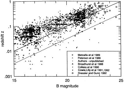
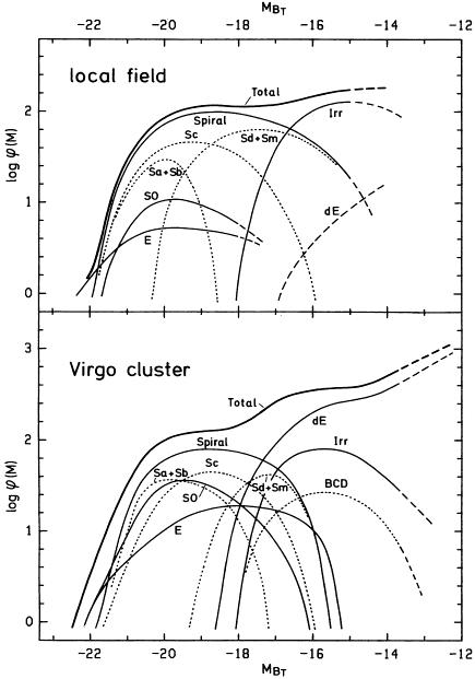
There are five needed ingredients. (1) The m = f(z) distribution giving the spread of apparent magnitude at given redshifts must be known. Typical distributions at various redshifts are set out in Fig. 13, taken from Koo and Kron (1992). (2) This distribution is the integral over morphological type of the type-dependent luminosity function as log N(M, type). An early example of such a luminosity function is shown in Fig. 14, based on both the Virgo Cluster survey and the local field (Binggeli, Sandage, and Tammann 1988) as defined by the Revised Shapley-Ames Catalog. (3) K corrections for any given band pass and morphological type, K(z, band pass, type), are needed to convert the Mattig equation in m(bol) to observed m(z). The SEDs for each galaxy type are needed to calculate these K corrections. Such calculations are given, among others, by Coleman, Wu, and Weedman (1980), and Yoshii and Takahara (1988). (4) The morphological type mix at each z is needed so as to add the separate calculations of N(m, type) to produce the composite N(m) over all types. A number of studies of the type mix as function of z are summarized elsewhere (Sandage 1988, section 7.2). (5) Faith, courage, and daring are needed to end with any conviction that the predicted N(m) describes reality, or, if the prediction disagrees with the observed N(m, band-pass) relations, that evolution (either density or luminosity, or both) as a function of both z and morphological type is required to make agreement. Much faith, courage, daring, and conviction have been displayed in the many current Journal papers concerning evolution in the look-back time. We shall see more of all four this week.

Figure 13. The distribution of redshift at given B apparent magnitudes from the various listed surveys. Diagram from Koo and Kron (1992).

Figure 14. Type-dependent luminosity function (H0 = 50) needed to calculate a realistic no-evolution N(m) predicted count-magnitude relation. Diagram from Binggeli et al. (1988).