We obtained long-slit spectra of the night sky using the Boller & Chivens Spectrograph on the 2.5m duPont Telescope at Las Campanas Observatory (LCO) on the nights of 1995 November 26-29. The first night of the run was lost to clouds. On the third night, a thermal short in the dewar caused poor temperature regulation of the CCD which resulted in low and variable charge transfer efficiency (see Section 3.1). The data from these two nights were therefore dropped from further analysis. The dewar was repaired for the remaining nights of the run. As discussed further in Section 3.3 and Section 3.6, both detector performance and photometric conditions were stable to better than 1% on the two useful nights of the run.
As described in Paper I, these spectra were taken within the field of view of our HST/WFPC2 observations, which executed in consecutive orbits on 1995 November 27-28. Because the HST and LCO observations executed simultaneously and along exactly the same pointing (see Paper I), the ZL contribution to both data sets is identical. The slit position is shown overlayed on a r-band image of the field in Figure 2. The exact coordinates of the spectroscopic observations were selected from ground-based imaging to avoid objects brighter than r = 26 mag arcsec-2. This was done for convenience in the data reduction; extragalactic sources need not be rigorously avoided, as spectral lines from extragalactic sources fainter than r ~ 24 AB mag will be significantly redshifted, on average, and should not align with solar features. In addition, such objects will have low enough surface number density (< 0.2 arcsec-2) that they will not significantly impact the average extracted spectrum.

|
Figure 2. The slit position during program observations. The image is a 4 × 4 arcmin2, r-band exposure taken the 2.5m duPont telescope at Las Campanas Observatory. WFPC2/HST observations were taken in parallel with the spectroscopy presented here for the purpose of measuring the EBL. For comparison, the WFPC2/HST field of view is also contained within this image, located towards the lower left quadrant (see Figure 7, Paper I). |
We used a 600 l/mm grating to obtain spectra over the wavelength range 3860-5150Å with a dispersion of ~ 1.3Å per pixel. The wavelength range was chosen to include a maximum number of strong Fraunhofer lines while avoiding strong airglow features. The strong MgIFraunhofer lines near ~ 5170Å were identified in an earlier run to be affected by rapidly variable airglow features and were therefore excluded from our 1995 spectral coverage. Ca H & K were included in our observations at the blue end. A slit-width of ~ 1.5arcsec (see Section 3.6.3) produced roughly 2.6Å resolution in the program observations. Even though the ZL has a surface brightness of µV ~ 23.2 mag arcsec-2, we obtained a signal-to-noise ratio of ~ 40 per spectral resolution element from a single, 30 minute exposure by integrating over the total slit surface area (~ 300arcsec2). To minimize read-noise, we binned the data on-chip by four pixels in the spatial direction and averaged over the full 3.4 arcmin spatial extent of the slit in the data reduction.
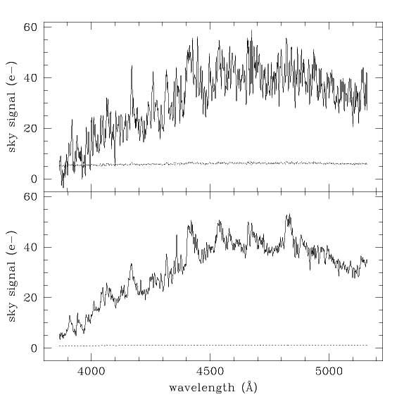
Spectrophotometric standards were observed through a slit 10.8arcsec wide. The detector we used is a thinned Tektronics/SITe CCD with 1024 × 1024 × 24µm pixels, 1.15e-/DN gain, and 8.6e- read-noise in the 4 × 1 binned configuration. The quantum efficiency of the CCD is near 50% over the spectral range of these observations; however, the spectrograph throughput drops by a factor of two between 5000Å and 3800Å, as can be seen from the sensitivity curve plotted in Figure 5. The upper panel of Figure 3 shows the wavelength calibrated spectrum obtained from one spatial resolution element (1 column) of one of the 4 × 1 binned exposures; the lower panel shows the averaged spectrum from the full image (87 columns). Above 4100Å, the count rate from sky is more than twice the dark rate. The maximum error is 10% per resolution element at the blue end of the spectra, simply due to the low count-rate at bluer wavelengths. Above 4100Å, the error per resolution element is roughly 1%.
|
Figure 3. Signal-to-noise of program data. The upper plot shows the wavelength-calibrated spectrum in electrons per pixel obtained from one spatial resolution element (column) of an 1800 second exposure of the night sky. The lower plot shows the spectrum produced by averaging 87 columns. The corresponding error spectra, both read-noise dominated, are shown with a dotted line at the bottom of each plot. |
Final calibration errors are summarized in Table 1. The data reduction steps are described below in the order which they were performed.