4.3.2. Magnetic fields from Higgs field equilibration

In the previous section we have seen that, concerning the generation of magnetic fields, the QCDPT and the EWPT share several common aspects. However, there is one important aspect which makes the EWPT much more interesting than the QCDPT. In fact, at the electroweak scale the electromagnetic field is directly influenced by the dynamics of the Higgs field which drives the EWPT.

To start with we remind that, as a consequence of the Weinberg-Salam theory, before the EWPT is not even possible to define the electromagnetic field, and that this operation remains highly non-trivial until the transition is completed. In a sense, we can say that the electromagnetic field was "born" during the EWPT. The main problem in the definition of the electromagnetic field at the weak scale is the breaking of the translational invariance: the Higgs field module and its SU(2) and U_Y(1) phases take different values in different positions. This is either a consequence of the presence of thermal fluctuations, which close to T_c are locally able to break/restore the SU(2) × U_Y(1) symmetry or of the presence of large stable domains, or bubbles, where the broken symmetry has settled.

The first generalized definition of the electromagnetic field in the presence of a non-trivial Higgs background was given by t'Hooft [149] in the seminal paper where he introduced magnetic monopoles in a SO(3) Georgi-Glashow model. t'Hooft definition is the following

(4.21)

In the above G ^a_µ W ^a_µ - W ^a, where

(4.22)

(^a are the Pauli matrices) is a unit isovector which defines the "direction" of the Higgs field in the SO(3) isospace (which coincides with SU(2)) and (D_µ)^a = _µ^a + g ^abc W_µ^bc, where W_µ^b are the gauge fields components in the adjoint representation. The nice features of the definition (4.21) are that it is gauge-invariant and it reduces to the standard definition of the electromagnetic field tensor if a gauge rotation can be performed so to have ^a = - ^a3 (unitary gauge). In some models, like that considered by t'Hooft, a topological obstruction may prevent this operation to be possible everywhere. In this case singular points (monopoles) or lines (strings) where ^a = 0 appear which become the source of magnetic fields. t'Hooft result provides an existence proof of magnetic fields produced by non-trivial vacuum configurations.

The Weinberg-Salam theory, which is based on the SU(2) × U_Y(1) group representation, does not predict topologically stable field configurations. We will see, however, that vacuum non-topological configurations possibly produced during the EWPT can still be the source of magnetic fields.

A possible generalization of the definition (4.21) for the Weinberg-Salam model was given by Vachaspati [106]. It is

(4.23)

D_µ = _µ - i[(g) / 2] ^a W_µ^a -i[(g') / 2] Y_µ.

This expression was used by Vachaspati to argue that magnetic fields should have been produced during the EWPT. Synthetically, Vachaspati argument is the following. It is known that well below the EWPT critical temperature T_c the minimum energy state of the Universe corresponds to a spatially homogeneous vacuum in which is covariantly constant, i.e. D = D_µ ^a = 0. However, during the EWPT, and immediately after it, thermal fluctuations give rise to a finite correlation length ~ (eT_c)^-1. Therefore, there are spatial variations both in the Higgs field module || and in its SU(2) and U(1)_Y phases which take random values in uncorrelated regions ⁽¹⁵⁾. It was noted by Davidson [150] that gradients in the radial part of the Higgs field cannot contribute to the production of magnetic fields as this component is electrically neutral. While this consideration is certainly correct, it does not imply the failure of Vachaspati argument. In fact, the role played by the spatial variations of the SU(2) and U(1)_Y "phases" of the the Higgs field cannot be disregarded. It is worthwhile to observe that gradients of these phases are not a mere gauge artifact as they correspond to a nonvanishing kinetic term in the Lagrangian. Of course one can always rotate Higgs fields phases into gauge boson degrees of freedom (see below) but this operation does not change F^em_µ which is a gauge-invariant quantity. The contribution to the electromagnetic field produced by gradients of ^a can be readily determined by writing the Maxwell equations in the presence of an inhomogeneous Higgs background [151]

(4.24)

Even neglecting the second term on the righthand side of Eq. (4.24), which depends on the definition of F^em_µ in a Higgs inhomogeneous background (see below), it is evident that a nonvanishing contribution to the electric 4-current arises from the covariant derivative of ^a. The physical meaning of this contribution may look more clear to the reader if we write Eq. (4.24) in the unitary gauge

(4.25)

Not surprisingly, we see that the electric currents produced by Higgs field equilibration after the EWPT are nothing but W boson currents.

Since, on dimensional grounds, D ~ v / where v is the Higgs field vacuum expectation value, Vachaspati concluded that magnetic fields (electric fields were supposed to be screened by the plasma) should have been produced at the EWPT with strength

(4.26)

Of course these fields live on a very small scale of the order of and in order to determine fields on a larger scale Vachaspati claimed that a suitable average has to be performed (see return on this issue below in this section).

Before discussing averages, however, let us try to understand better the nature of the magnetic fields which may have been produced by the Vachaspati mechanism. We notice that Vachaspati's derivation does not seem to invoke any out-of-equilibrium process and indeed the reader may wonder what is the role played by the phase transition in the magnetogenesis. Moreover, magnetic fields are produced anyway on a scale (eT)^-1 by thermal fluctuations of the gauge fields so that it is unclear what is the difference between magnetic fields produced by the Higgs fields equilibration and these more conventional fields. In our opinion, although Vachaspati's argument is basically correct its formulation was probably oversimplified. Indeed, several works showed that in order to reach a complete understanding of this physical effect a more careful study of the dynamics of the phase transition is called for. We shall now review these works starting from the case of a first order phase transition.

The case of a first order EWPT

Before discussing the SU(2) × U(1) case we cannot overlook some important work which was previously done about phase equilibration during bubble collision in the framework of more simple models. In the context of a U(1) Abelian gauge symmetry, Kibble and Vilenkin [152] showed that the process of phase equilibration during bubble collisions give rise to relevant physical effects. The main tool developed by Kibble and Vilenkin to investigate this kind of processes is the, so-called, gauge-invariant phase difference defined by

(4.27)

where is the U(1) Higgs field phase and D_{µ µ} + e A_µ is the phase covariant derivative. A and B are points taken in the bubble interiors and k = 1,2,3. obeys the Klein-Gordon equation

(4.28)

where m = ev is the gauge boson mass. Kibble and Vilenkin assumed that during the collision the radial mode of the Higgs field is strongly damped so that it rapidly settles to its expectation value v everywhere. One can choose a frame of reference in which the bubbles are nucleated simultaneously with centers at (t, x, y, z) = (0,0,0, ± R_c). In this frame, the bubbles have equal initial radius R_i = R₀. Their first collision occurs at (t_c, 0, 0, 0) when their radii are R_c and t_c = sqrt[R_c² - R₀²]. Given the symmetry of the problem about the axis joining the nucleation centers (z-axis), the most natural gauge is the axial gauge. In this gauge

(4.29)

where = 0, 1, 2 and ² = t² - x² - y² . The condition _a(, 0) = 0 fixes the gauge completely. At the point of first contact z = 0, = t_c the Higgs field phase was assumed to change from ₀ to -₀ going from a bubble into the other. This constitutes the initial condition of the problem. The following evolution of is determined by the Maxwell equation

(4.30)

and the Klein-Gordon equation which splits into

	(4.31)
	(4.32)

The solution of the linearized equations (4.31) and (4.32) for > t_c then becomes

	(4.33)
	(4.34)

where ² = k²+m². The gauge-invariant phase difference is deduced by the asymptotic behavior at z ±

(4.35)

Thus, phase equilibration occurs with a time scale t_c determined by the bubble size, with superimposed oscillations with frequency given by the gauge-field mass. As we see from Eq. (4.34) phase oscillations come together with oscillations of the gauge field. It follows from Eq. (4.30) that these oscillations give rise to an "electric" current. This current will source an "electromagnetic" field strength F_µ ⁽¹⁶⁾. Because of the symmetry of the problem the only nonvanishing component of F_µ is

(4.36)

Therefore, we have an azimuthal magnetic field B = F ^z = _z a and a longitudinal electric field E^z = F^0z = -t_z a = -(t / ) B(, z), where we have used cylindrical coordinates (, ). We see that phase equilibration during bubble collision indeed produces some real physical effects.

Kibble and Vilenkin did also consider the role of electric dissipation. They showed that a finite value of the electric conductivity gives rise to a damping in the "electric" current which turns into a damping for the phase equilibration. They found

(4.37)

for small values of , and

(4.38)

in the opposite case. The dissipation time scale is typically much smaller than the time which is required for two colliding bubble to merge completely. Therefore the gauge-invariant phase difference settles rapidly to zero in the overlapping region of the two bubbles and in its neighborhood. It is interesting to compute the line integral of D_k over the path ABCD represented in the Fig. 4.1.

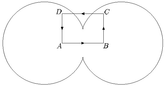
Figure 4.1. Two colliding bubbles. It is showed the closed path along which the displacement of the gauge invariant phase difference is computed. (From Ref. [152]).

From the previous considerations it follows that _AB = 0, _AD = _BC = 0 and _DC = 2₀. It is understood that in order for the integral to be meaningful, the vacuum expectation value of the Higgs field has to remain nonzero in the collision region and around it, so that the phase remains well defined and interpolates smoothly between its values inside the bubbles. Under these hypothesis we have

(4.39)

The physical meaning of this quantity is recognizable at a glance in the unitary gauge, in which each is given by a line integral of the vector potential A. We see that the gauge-invariant phase difference computed along the loop is nothing but the magnetic flux trough the loop itself

(4.40)

In other words, phase equilibration give rise to a ring of magnetic flux near the circle on which bubble walls intersect. If the initial phase difference between the two bubbles is 2, the total flux trapped in the ring is exactly one flux quantum, 2 / e.

Kibble and Vilenkin did also consider the case in which three bubbles collide. They argued that in this case the formation of a string, in which interior symmetry is restored, is possible. Whether or not this happens is determined by the net phase variation along a closed path going through the three bubbles. The string forms if this quantity is larger than 2. According to Kibble and Vilenkin strings cannot be produced by two bubble collisions because, for energetic reasons, the system will tend to choose the shorter of the two paths between the bubble phases so that a phase displacement 2 can never be obtained. This argument, which was first used by Kibble [153] for the study of defect formation, is often called the "geodesic rule".

The work of Kibble and Vilenkin was reconsidered by Copeland and Saffin [154] and more recently by Copeland, Saffin and Törnkvist [155] who showed that during bubble collision the dynamics of the radial mode of the Higgs field cannot really be disregarded. In fact, violent fluctuations in the modulus of the Higgs field take place and cause symmetries to be restored locally, allowing the phase to "slip" by an integer multiple of 2 violating the geodesic rule. Therefore strings, which carry a magnetic flux, can be produced also by the collision of only two bubbles. Saffin and Copeland [156] went a step further by considering phase equilibration in the SU(2) × U(1) case, namely the electroweak case. They showed that for some particular initial conditions the SU(2) × U(1) Lagrangian is equivalent to a U(1) Lagrangian so that part of Kibble and Vilenkin [152] considerations can be applied. The violation of the geodesic rule allows the formation of vortex configurations of the gauge fields. Saffin and Copeland argued that these configurations are related to the Nielsen-Olesen vortices [157]. Indeed, it is know that such a kind of non-perturbative solutions are allowed by the Weinberg-Salam model [158] (for a comprehensive review on electroweak strings see Ref. [159]). Although electroweak string are not topologically stable, numerical simulations performed in Ref. [156] show that in presence of small perturbations the vortices survives on times comparable to the time required for bubble to merge completely.

The generation of magnetic fields in the SU(2) × U(1)_Y case was not considered in the work by Saffin and Copeland. This issue was the subject of a following paper by Grasso and Riotto [151]. The authors of Ref. [151] studied the dynamics of the gauge fields starting from the following initial Higgs field configuration

(4.41)

which represents the superposition of the Higgs fields of two bubbles which are separated by a distance b. In the above n^a is a unit vector in the SU(2) isospace and ^a are the Pauli matrices. The phases and the orientation of the Higgs field were chosen to be uniform across any single bubble. It was assumed that Eq. (4.41) holds until the two bubble collide (t = 0). Since n^{a a} is the only Lie-algebra direction which is involved before the collision, one can write the initial Higgs field configuration in the form [156]

(4.42)

In order to disentangle the peculiar role played by the Higgs field phases, the initial gauge fields W_µ^a and their derivatives were assumed to be zero at t = 0. This condition is of course gauge dependent and should be interpreted as a gauge choice. It is convenient to write the equation of motion for the gauge fields in the adjoint representation. For the SU(2) gauge fields we have

(4.43)

where the isovector ^a has been defined in Eq. (4.22). Under the assumptions mentioned in the above, at t = 0, this equation reads

(4.44)

In general, the unit isovector ^a can be decomposed into

(4.45)

where ^T₀ - (0, 0, 1). It is straightforward to verify that in the unitary gauge, reduces to ₀. The relevant point in Eq. (4.42) is that the versor [^(n)], about which it is performed the SU(2) gauge rotation, does not depend on the space coordinates. Therefore, without loosing generality, we have the freedom to choose to be everywhere perpendicular to ₀. In other words, can be everywhere obtained by rotating ₀ by an angle in the plane identified by and ₀. Formally, = cos ₀ + sin × ₀, which clearly describes a simple U(1) transformation. In fact, since it is evident that the condition ₀ also implies , the equation of motion (4.44) becomes

(4.46)

As expected, we see that only the gauge field component along the direction , namely A_µ = n^a W^a_µ, that has some initial dynamics which is created by a nonvanishing gradient of the phase between the two domains. When we generalize this result to the full SU(2) × U(1)_Y gauge structure, an extra generator, namely the hypercharge, comes-in. Therefore in this case is not any more possible to choose an arbitrary direction for the unit vector since different orientations of the unit vector with respect to ₀ correspond to different physical situations. We can still consider the case in which is parallel to ₀ but we should take in mind that this is not the only possibility. In this case we have

	(4.47)
	(4.48)

where g and g' are respectively the SU(2) and U(1)_Y gauge coupling constants. It is noticeable that in this case the charged gauge fields are not excited by the phase gradients at the time when bubble first collide. We can combine Eqs. (4.47) and (4.48) to obtain the equation of motion for the Z-boson field

(4.49)

This equation tells us that a gradient in the phases of the Higgs field gives rise to a nontrivial dynamics of the Z-field with an effective gauge coupling constant sqrt[g² + g^'2]. We see that the equilibration of the phase ( + ) can be now treated in analogy to the U(1) toy model studied by Kibble and Vilenkin [152], the role of the U(1) "electromagnetic" field being now played by the Z-field. However, differently from Ref. [152] the authors of Ref. [151] left the Higgs field modulus free to change in space. Therefore, the equation of motion of (x) has to be added to (4.49). Assuming the charged gauge field does not evolve significantly, the complete set of equations of motion that we can write at finite, though small, time after the bubbles first contact, is

(4.50)

where d_µ = _µ + i[g / (2cos_W)] Z_µ, is the vacuum expectation value of and is the quartic coupling. Note that, in analogy with [152], a gauge invariant phase difference can be introduced by making use of the covariant derivative d_µ. Equations (4.50) are the Nielsen-Olesen equations of motion [157]. Their solution describes a Z-vortex where = 0 at its core [160]. The geometry of the problem implies that the vortex is closed, forming a ring which axis coincide with the conjunction of bubble centers. This result provides further support to the possibility that electroweak strings are produced during the EWPT.

In principle, in order to determine the magnetic field produced during the process that we illustrated in the above, we need a gauge-invariant definition of the electromagnetic field strength in the presence of the non-trivial Higgs background. We know however that such definition is not unique [161]. For example, the authors of Ref. [151] used the definition given in Eq. (4.23) to find that the electric current is

(4.51)

whereas other authors [162], using the definition

(4.52)

found no electric current, hence no magnetic field, at all. We have to observe, however, that the choice between these, as others, gauge invariant definitions is more a matter of taste than physics. Different definitions just give the same name to different combinations of the gauge fields. The important requirement which acceptable definitions of the electromagnetic field have to fulfill is that they have to reproduce the standard definition in the broken phase with a uniform Higgs background. This requirement is fulfilled by both the definitions used in the Refs. [151] and [162]. In our opinion, it is not really meaningful to ask what is the electromagnetic field inside, or very close to, the electroweak strings. The physically relevant question is what are the electromagnetic relics of the electroweak strings once the EWPT is concluded.

One important point to take in mind is that electroweak strings are not topologically stable (see [159] and references therein) and that, for the physical value of the Weinberg angle, they rapidly decay after their formation. Depending on the nature of the decay process two scenarios are possible. According to Vachaspati [163] long strings should decay in short segments of length ~ m_W^-1. Since the Z-string carry a flux of Z-magnetic flux in its interior

(4.53)

and the Z gauge field is a linear superposition of the W³ and Y fields then, when the string terminates, the Y flux cannot terminate because it is a U(1) gauge field and the Y magnetic field is divergenceless. Therefore some field must continue even beyond the end of the string. This has to be the massless field of the theory, that is, the electromagnetic field. In some sense, a finite segment of Z-string terminates on magnetic monopoles [158]. The magnetic flux emanating from a monopole is:

(4.54)

This flux may remain frozen-in the surrounding plasma and become a seed for cosmological magnetic fields.

Another possibility is that Z-strings decay by the formation of a W-condensate in their cores. In fact, it was showed by Perkins [164] that while electroweak symmetry restoration in the core of the string reduces m_W, the magnetic field via its coupling to the anomalous magnetic moment of the W-field, causes, for eB > m_W², the formation of a condensate of the W-fields. Such a process is based on the Ambj orn-Olesen instability which will be discussed in some detail in the Chap.5 of this review. As noted in [151] the presence of an inhomogeneous W-condensate produced by string decay gives rise to electric currents which may sustain magnetic fields even after the Z string has disappeared. The formation of a W-condensate by strong magnetic fields at the EWPT time, was also considered by Olesen [165].

We can now wonder what is the predicted strength of the magnetic fields at the end of the EWPT. An attempt to answer to this question has been done by Ahonen and Enqvist [166] (see also Ref. [167]) where the formation of ring-like magnetic fields in collisions of bubbles of broken phase in an Abelian Higgs model were inspected. Under the assumption that magnetic fields are generated by a process that resembles the Kibble and Vilenkin [152] mechanism, it was concluded that a magnetic field of the order of B 2 × 10²⁰ G with a coherence length of about 10² GeV^-1 may be originated. Assuming turbulent enhancement the authors of Ref. [166] of the field by inverse cascade [51], a root-mean-square value of the magnetic field B_rms 10^-21 G on a comoving scale of 10 Mpc might be present today. Although our previous considerations give some partial support to the scenario advocated in [166] we have to stress, however, that only in some restricted cases it is possible to reduce the dynamics of the system to the dynamics of a simple U(1) Abelian group. Furthermore, once Z-vortices are formed the non-Abelian nature of the electroweak theory shows due to the back-reaction of the magnetic field on the charged gauge bosons and it is not evident that the same numerical values obtained in [166] will be obtained in the case of the EWPT.

However the most serious problem with the kind of scenario discussed in this section comes form the fact that, within the framework of the standard model, a first order EWPT seems to be incompatible with the Higgs mass experimental lower limit [143]. Although some parameter choice of the minimal supersymmetric standard model (MSSM) may still allow a first order transition [144], which may give rise to magnetic fields in a way similar to that discussed in the above, we think it is worthwhile to keep an open mind and consider what may happen in the case of a second order transition or even in the case of a cross over.

The case of a second order EWPT

As we discussed in the first part of this section, magnetic fields generation by Higgs field equilibration share several common aspects with the formation of topological defects in the early Universe. This analogy holds, and it is even more evident, in the case of a second order transition. The theory of defect formation during a second order phase transition was developed in a seminal paper by Kibble [153]. We shortly review some relevant aspects of the Kibble mechanism. We start from the Universe being in the unbroken phase of a given symmetry group G. As the Universe cools and approach the critical temperature T_c protodomains are formed by thermal fluctuations where the vacuum is in one of the degenerate, classically equivalent, broken symmetry vacuum states. Let M be the manifold of the broken symmetry degenerate vacua. The protodomains size is determined by the Higgs field correlation function. Protodomains become stable to thermal fluctuations when their free energy becomes larger than the temperature. The temperature at which this happens is usually named Ginsburg temperature T_G. Below T_G stable domains are formed which, in the case of a topologically nontrivial manifold M, give rise to defect production. Rather, if M is topologically trivial, phase equilibration will continue until the Higgs field is uniform everywhere. This is the case of the Weinberg-Salam model, as well as of its minimal supersymmetrical extension.

Higgs phase equilibration, which occurs when stable domains merge, gives rise to magnetic fields in a way similar to that described by Vachaspati [106] (see the beginning of this section). One should keep in mind, however, that as a matter of principle, the domain size, which determine the Higgs field gradient, is different from the correlation length at the critical temperature [151]. At the time when stable domains form, their size is given by the correlation length in the broken phase at the Ginsburg temperature. This temperature was computed, in the case of the EWPT, by the authors of Ref. [151] by comparing the expansion rate of the Universe with the nucleation rate per unit volume of sub-critical bubbles of symmetric phase (with size equal to the correlation length in the broken phase) given by

(4.55)

where l_b is the correlation length in the broken phase. S₃^ub is the high temperature limit of the Euclidean action (see e.g. Ref. [168]). It was shown that for the EWPT the Ginsburg temperature is very close to the critical temperature, T_G = T_c within a few percent. The corresponding size of a broken phase domain is determined by the correlation length in the broken phase at T = T_G

(4.56)

where V(, T) is the effective Higgs potential. (T_G)²_b is weakly dependent on M_H, _b(T_G) 11/ T_G for M_H = 100 GeV and _b(T_G) 10 / T_G for M_H = 200 GeV. Using this result and Eq. (4.23) the authors of Ref. [151] estimated the magnetic field strength at the end of the EWPT to be of order of

(4.57)

on a length scale _b(T_G).

Although it was showed by Martin and Davis [169] that magnetic fields produced on such a scale may be stable against thermal fluctuations, it is clear that magnetic fields of phenomenological interest live on scales much larger than _b(T_G). Therefore, some kind of average is required. We are ready to return to the discussion of the Vachaspati mechanism for magnetic field generation [106]. Let us suppose we are interested in the magnetic field on a scale L = N . Vachaspati argued that, since the Higgs field is uncorrelated on scales larger than , its gradient executes a random walk as we move along a line crossing N domains. Therefore, the average of the gradient D_µ over this path should scale as N. Since the magnetic field is proportional to the product of two covariant derivatives, see Eq. (4.23), Vachaspati concluded that it scales as 1 / N. This conclusion, however, overlooks the difference between <D_µ ^†> <D_µ ;> and <D_µ ^† D_µ >. This point was noticed by Enqvist and Olesen [107] (see also Ref. [109]) who produced a different estimate for the average magnetic field, <B>_{rms, L} B(L) ~ B / N. Neglecting the possible role of the magnetic helicity (see the next section) and of possible related effects, e.g. inverse cascade, and using Eq. (4.57), the line-averaged field today on a scale L ~ 1 Mpc (N ~ 10²⁵) is found to be of the order B₀(1 Mpc) ~ 10^-21 G.

Another important point of this kind of scenario (for the reasons which will become clear in the next section) is that it naturally gives rise to a nonvanishing vorticity. This point can be understood by the analogy with the process which lead to the formation of superfluid circulation in a Bose-Einstein fluid which is rapidly taken below the critical point by a pressure quench [170]. Consider a circular closed path through the superfluid of length C = 2R. This path will cross N C / domains, where is the characteristic size of a single domain. Assuming that the phase of the condensate wave function is uncorrelated in each of the N domains (random-walk hypothesis) the typical mismatch of is given by:

(4.58)

where is the phase gradient across two adjacent domains and ds is the line element along the circumference. It is well known (see e.g. [171]) that from the Schrödinger equation it follows that the velocity of a superfluid is given by the gradient of the phase trough the relation v_s = ( / m) , therefore (4.58) implies

(4.59)

It was argued by Zurek [170] that this phenomenon can effectively simulate the formation of defects in the early Universe. As we discussed in the previous section, although the standard model does not allows topological defects, embedded defects, namely electroweak strings, may be produced through a similar mechanism. Indeed a close analogy was showed to exist [172] between the EWPT and the ³He superfluid transition where formation of vortices is experimentally observed. This hypothesis received further support by some recent lattice simulations which showed evidence for the formation of a cluster of Z-strings just above the cross-over temperature [173] in the case of a 3D SU(2) Higgs model. Electroweak strings should lead to the generation of magnetic fields in the same way we discussed in the case of a first order EWPT. Unfortunately, to estimate the strength of the magnetic field produced by this mechanism requires the knowledge of the string density and net helicity which, so far, are rather unknown quantities.

¹⁵ Vachaspati [106] did also consider Higgs field gradients produced by the presence of the cosmological horizon. However, since the Hubble radius at the EWPT is of the order of 1 cm whereas ~ (eT_c)^-1 ~ 10^-16 cm, it is easy to realize that magnetic fields possibly produced by the presence of the cosmological horizon are phenomenologically irrelevant. Back.

¹⁶ It is understood that since the toy model considered by Kibble e Vilenkin is not SU(2) × U(1)_Y, F_µ is not the physical electromagnetic field strength. Back.