


The preceding section was devoted to the case in which one had a discrete set of hypotheses among which to choose. It is more common in physics to have an infinite set of hypotheses; i.e., a parameter that is a continuous variable. For example, in the µ-e decay distribution
|
the possible values for
 0 belong to a
continuous rather than a
discrete set. In this case, as before, we invoke the same basic
principle which says the relative probability of any two different
values of is the ratio of
the probabilities of getting our
particular experimental results, xi, assuming first
one and then
the other, value of is
true. This probability function of
is called the likelihood function,
0 belong to a
continuous rather than a
discrete set. In this case, as before, we invoke the same basic
principle which says the relative probability of any two different
values of is the ratio of
the probabilities of getting our
particular experimental results, xi, assuming first
one and then
the other, value of is
true. This probability function of
is called the likelihood function,
 ().
().
| (2) |
The likelihood function,
| |
| |
The relative probabilities of
can be displayed as a plot of
() vs.
. The most probable value of
is
called the maximum-likelihood solution
*. The rms (root-mean-square)
spread of about
* is a conventional measure
of the accuracy of the
determination =
* . We shall call this
 .
.
| (3) |
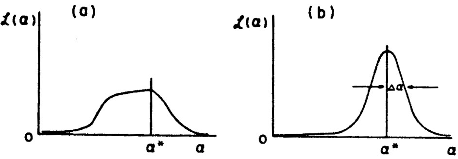
In general, the likelihood function will be close to Gaussian
(it can be shown to approach a Gaussian distribution as
N ->  )
and will look similar to Fig. 1b.
)
and will look similar to Fig. 1b.
Fig. 1a represents what is called a case of poor
statistics. In
such a case, it is better to present a plot of
() rather than merely quoting
* and
. Straightforward
procedures for obtaining
are presented in
Sections 6 and 7.
|
Figure 1. Two examples of likelihood
functions |
A confirmation of this inverse probability approach is the
Maximum-Likelihood Theorem, which is proved in Cramer
[4] by use
of direct probability. The theorem states that in the limit of
large N,
* ->
0; and
furthermore, there is
no other method of estimation that is more accurate.
In the general case in which there are M parameters,
1, ...,
M, to be
determined, the procedure for obtaining the
maximum likelihood solution is to solve the M simultaneous
equations,
| (4) |