


We have seen that inflation is a powerful and predictive theory of the physics of the very early universe. Unexplained properties of a standard FRW cosmology, namely the flatness and homogeneity of the universe, are natural outcomes of an inflationary expansion. Furthermore, inflation provides a mechanism for generating the tiny primordial density fluctuations that seed the later formation of structure in the universe. Inflation makes definite predictions, which can be tested by precision observation of fluctuations in the CMB, a program that is already well underway.
In this section, we will move beyond looking at inflation as a subject
of experimental test
and discuss some intriguing new ideas that indicate that inflation might
be useful as a tool
to illuminate physics at extremely high energies, possibly up to the
point where effects
from quantum gravity become relevant. This idea is based on a simple
observation about scales in the universe. As we discussed in
Sec. 2, quantum field theory extended to
infinitely high energy scales gives nonsensical (i.e., divergent)
results. We therefore
expect the theory to break down at high energy, or equivalently at very
short lengths. We
can estimate the length scale at which quantum mechanical effects from
gravity become
important by simple dimensional analysis. We define the Planck length
 Pl
by an appropriate combination of fundamental constants as
Pl
by an appropriate combination of fundamental constants as
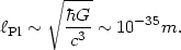 |
(133) |
For processes probing length scales shorter than
Pl, such as
quantum modes with wavelengths
 <
Pl, we expect
some sort of new physics to be important.
There are a number of ideas for what that new physics might be, for
example string theory
or noncommutative geometry or discrete spacetime, but physics at the
Planck scale is currently
not well understood. It is unlikely that particle accelerators will
provide insight into
such high energy scales, since quantum modes with wavelengths less than
Pl will
be characterized by energies of order
1019 GeV or so, and current particle
accelerators operate at energies around 103 GeV.
(12)
However, we note an interesting
fact, namely that the ratio between the current horizon size of the
universe and the Planck length is about
<
Pl, we expect
some sort of new physics to be important.
There are a number of ideas for what that new physics might be, for
example string theory
or noncommutative geometry or discrete spacetime, but physics at the
Planck scale is currently
not well understood. It is unlikely that particle accelerators will
provide insight into
such high energy scales, since quantum modes with wavelengths less than
Pl will
be characterized by energies of order
1019 GeV or so, and current particle
accelerators operate at energies around 103 GeV.
(12)
However, we note an interesting
fact, namely that the ratio between the current horizon size of the
universe and the Planck length is about
 |
(134) |
or, on a log scale,
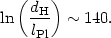 |
(135) |
This is a big number, but we recall our earlier discussion of the
flatness and horizon problems
and note that inflation, in order to adequately explain the flatness and
homogeneity of the
universe, requires the scale factor to increase by at least a
factor of e55. Typical
models of inflation predict much more expansion, e1000
or more. We remember that the
wavelength of quantum modes created during the inflationary expansion,
such as those responsible
for density and gravitational-wave fluctuations, have wavelengths which
redshift proportional to the scale factor, so that so that the
wavelength i
of a mode at early times can be given in terms of its wavelength
0 today by
 |
(136) |
This means that if inflation lasts for more than about N ~ 140 e-folds, fluctuations of order the size of the universe today were smaller than the Planck length during inflation! This suggests the possibility that Plank-scale physics might have been important for the generation of quantum modes in inflation. The effects of such physics might be imprinted in the pattern of cosmological fluctuations we see in the CMB and large-scale structure today. In what follows, we will look at the generation of quantum fluctuations in inflation in detail, and estimate how large the effect of quantum gravity might be on the primordial power spectrum.
In Sec. 2.4 we saw that the state space for
a quantum field theory was a set of states
(n(k1), ..., n(ki))
representing the number of particles with momenta
k1,...,ki. The creation and annihilation
operators  †k and
k act on
these states by adding or subtracting a particle from the state:
†k and
k act on
these states by adding or subtracting a particle from the state:
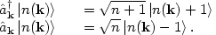 |
(137) |
The ground state, or vacuum state of the space is just the zero particle state,
 |
(138) |
Note in particular that the vacuum state |0> is not equivalent to zero. The vacuum is not nothing:
 |
(139) |
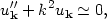
To construct a quantum field, we look at the familiar classical wave equation for a scalar field,
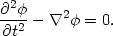 |
(140) |
To solve this equation, we decompose into Fourier modes uk,
 |
(141) |
where the mode functions uk(t) satisfy the ordinary differential equations
 |
(142) |
This is a classical wave equation with a classical solution, and the Fourier coefficients ak are just complex numbers. The solution for the mode function is
 |
(143) |
where  k
satisfies the dispersion relation
k
satisfies the dispersion relation
 |
(144) |
To turn this into a quantum field, we identify the Fourier coefficients with creation and annihilation operators
 |
(145) |
and enforce the commutation relations
 |
(146) |
This is the standard quantization of a scalar field in Minkowski space, which should be familiar. But what probably isn't familiar is that this solution has an interesting symmetry. Suppose we define a new mode function uk which is a rotation of the solution (143):
 |
(147) |
This is also a perfectly valid solution to the original wave
equation (140), since it is just a superposition of the Fourier
modes. But we can then re-write the quantum
field in terms of our original Fourier modes and new operators
 k and
†k and the original Fourier
modes eik . x as:
k and
†k and the original Fourier
modes eik . x as:
 |
(148) |
where the new operators
k are
given in terms of the old operators
k by
 |
(149) |
This is completely equivalent to our original solution (141) as long as the new operators satisfy the same commutation relation as the original operators,
 |
(150) |
This can be shown to place a condition on the coefficients A and B,
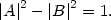 |
(151) |
Otherwise, we are free to choose A and B as we please.
This is just a standard property of linear differential equations: any
linear combination of
solutions is itself a solution. But what does it mean physically? In one
case, we have an annihilation operator
k which
gives zero when acting on a particular state which
we call the vacuum state:
 |
(152) |
Similarly, our rotated operator
k gives
zero when acting on some state
 |
(153) |
The point is that the two "vacuum" states are not the same
 |
(154) |
From this point of view, we can define any state we wish to be the
"vacuum" and build a
completely consistent quantum field theory based on this
assumption. From another equally
valid point of view this state will contain particles. How do we tell
which is the
physical vacuum state? To define the real vacuum, we have to
consider the spacetime
the field is living in. For example, in regular special relativistic
quantum field theory,
the "true" vacuum is the zero-particle state as seen by an inertial
observer. Another
more formal way to state this is that we require the vacuum to be
Lorentz symmetric. This fixes our choice of vacuum
|0> and defines unambiguously our set of creation and annihilation
operators and
†. A
consequence of this is that
an accelerated observer in the Minkowski vacuum will think that
the space is full of particles, a phenomenon known as the Unruh effect
[43].
The zero-particle state for an accelerated observer is different than
for an inertial observer.
So far we have been working within the context of field theory in special relativity. What about in an expanding universe? The generalization to a curved spacetime is straightforward, if a bit mysterious. We will replace the metric for special relativity with a Robertson-Walker metric,
 |
(155) |
Note that we have written the Robertson-Walker metric in terms of
conformal time
d = dt/a.
This is convenient for doing field theory, because the new spacetime is
just a Minkowski
space with a time-dependent conformal factor out front. In fact we
define the physical vacuum
in a similar way to how we did it for special relativity: the vacuum is
the zero-particle
state as seen by a geodesic observer, that is, one in free-fall
in the expanding
space. This is referred to as the Bunch-Davies vacuum.
= dt/a.
This is convenient for doing field theory, because the new spacetime is
just a Minkowski
space with a time-dependent conformal factor out front. In fact we
define the physical vacuum
in a similar way to how we did it for special relativity: the vacuum is
the zero-particle
state as seen by a geodesic observer, that is, one in free-fall
in the expanding
space. This is referred to as the Bunch-Davies vacuum.
Now we write down the wave equation for a free field, the equivalent of Eq. (140) in a Robertson-Walker space. This is the usual equation with a new term that comes from the expansion of the universe:
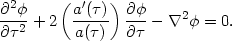 |
(156) |
Note that the time derivatives are with respect to the conformal time
, not the coordinate
time t. As in the Minkowski case, we Fourier expand the field,
but with an extra factor
of a() in the integral:
 |
(157) |
Here k is a comoving wavenumber (or, equivalently, momentum),
which stays constant as the mode redshifts with the expansion
 a, so that
 |
(158) |
Writing things this way, in terms of conformal time and comoving
wavenumber, makes the equation of motion for the mode
uk()
very similar to the mode equation (142) in Minkowski space:
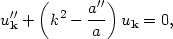 |
(159) |
where a prime denotes a derivative with respect to conformal time. All
of the effect of the
expansion is in the a"/a term. (Be careful not to
confuse the scale factor
a() with
the creation/annihilation operators
k and
†k!)
This equation is easy to solve. First consider the short wavelength limit, that is large wavenumber k. For k2 >> a"/a, the mode equation is just what we had for Minkowski space
 |
(160) |
except that we are now working with comoving momentum and conformal time, so the space is only quasi-Minkowski. The general solution for the mode is
 |
(161) |
Here is where the definition of the vacuum comes in. Selecting the
Bunch-Davies vacuum is
equivalent to setting A = 1 and B = 0, so that the
annihilation operator is multiplied by
e-ik and
not some linear combination of positive and negative frequencies. This
is the exact analog of Eq. (147). So the mode function corresponding to
the zero-particle state for an observer in free fall is
 |
(162) |
What about the long wavelength limit, k2 << a"/a? The mode equation becomes trivial:
 |
(163) |
with solution
 |
(164) |
The mode is said to be frozen at long wavelengths, since the
oscillatory behavior is
damped. This is precisely the origin of the density and gravity-wave
fluctuations in inflation.
Modes at short wavelengths are rapidly redshifted by the inflationary
expansion so that the
wavelength of the mode is larger than the horizon size, Eq. (164). We
can plot the mode as a function of its physical wavelength
= k/a
divided by the horizon size dH = H-1
(Fig. 19), and find that at
long wavelengths, the mode freezes out to a nonzero value.
 |
Figure 19. The mode function
uk / a as a function of
dH /
|
The power spectrum of fluctuations is just given by the two-point correlation function of the field,
 |
(165) |
This means that we have produced classical perturbations at long wavelength from quantum fluctuations at short wavelength.
What does any of this have to do with quantum gravity? Remember that we
have seen that for
an inflationary period that lasts longer than 140 e-folds or so, the
fluctuations we see
with wavelengths comparable to the horizon size today started out with
wavelengths shorter than the Planck length
Pl ~
10-35 cm during inflation. For a mode with
a wavelength that short, do we really know how to select the "vacuum"
state, which we
have assumed is given by Eq. (162)? Not necessarily. We do know that once
the mode redshifts to a wavelength greater than
Pl, it must be of
the form (161), but we know longer know for certain how to select the values
of the constants A(k) and B(k). What we have
done is mapped the effect of quantum gravity onto
a boundary condition for the mode function
uk. In principle, A(k) and
B(k) could
be anything! If we allow A and B to remain arbitrary, it
is simple to calculate the
change in the two-point correlation function at long wavelength,
 |
(166) |
where the subscript B-D indicates the value for the case of the "standard" Bunch-Davies vacuum, which corresponds to the choice A = 1, B = 0. So the power spectrum of gravity-wave and density fluctuations is sensitive to how we choose the vacuum state at distances shorter than the Planck scale, and is in principle sensitive to quantum gravity.
While in principle A(k) and B(k) are arbitrary, a great deal of recent work has been done implementing this idea within the context of reasonable toy models of the physics of short distances. There is some disagreement in the literature with regard to how big the parameter B can reasonably be. As one might expect on dimensional grounds, the size of the rotation is determined by the dimensionless ratio of the Planck length to the horizon size, so it is expected to be small
 |
(167) |
Here we have introduced a power p on the ratio, which varies depending on which model of short-distance physics you choose. Several groups have shown an effect linear in the ratio, p = 1. Fig. 20 shows the modulation of the power spectrum calculated in the context of one simple model [44].
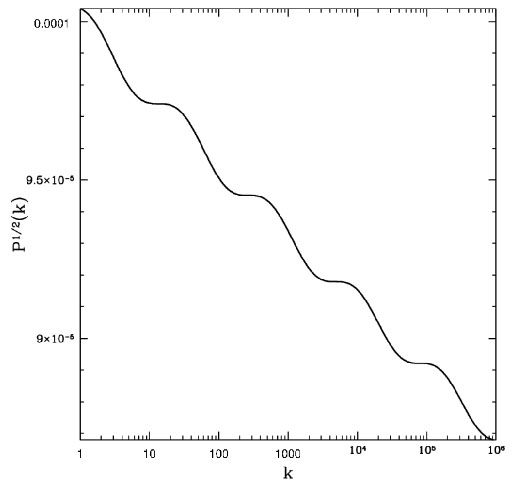 |
Figure 20. Modulation of the power spectrum of primordial fluctuations for a rotation B ~ H/mPl. |
Others have argued that this is too optimistic, and that a more realistic estimate is p = 2 [45] or even smaller [46]. The difference is important: if p = 1, the modulation of the power spectrum can be as large as a percent or so, a potentially observable value [47]. Take p = 2 and the modulation drops to a hundredth of a percent, far too small to see. Nonetheless, it is almost certainly worth looking for!
12 This might not be so in "braneworld" scenarios where the energy scale of quantum gravity can be much lower [42]. Back.