6.2. Comparison between the GPS/CSS and the LRL 3CR

O'Dea & Baum (1997) have shown that at 5 GHz in the rest frame, the Stanghellini GPS and Fanti CSS sources are just as powerful as the 3CR in the Laing, Riley, & Longair (1983, hereafter LRL) revised sample. These GPS and CSS sources would apparently have been in the LRL 3CR if their spectra did not turn over. The power versus size plot was introduced by Baldwin (1982) as a tool with which to study radio source evolution. O'Dea & Baum plot power versus projected largest linear size (Fig. 12) for the complete GPS and CSS samples and the LRL 3CR for the redshift range 0.2 z 1.0, where there is good overlap between the samples. At this range of redshifts, the LRL 3CR sources are almost exclusively classical doubles. Out to sizes of several kpc, the power is constant with size, and at larger sizes the power may decline slightly with increasing size (cf. Leahy & Williams 1984; Nilsson et al. 1993; Readhead et al. 1996a).

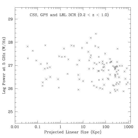Figure 12. The log of power at 5 GHz vs. the projected linear size for sources in the redshift range 0.2 z 1.0 from the LRL 3CR and the Fanti et al. CSS sample and the Stanghellini et al. GPS sample. Adapted from O'Dea & Baum (1997).

The P-l diagram is a "snapshot" of radio source evolution, and individual sources will trace out trajectories in the P-l plane as they evolve. A constraint on radio source evolution comes from the number of sources as a function of size in the P-l plane. O'Dea & Baum plot the number of sources in bins of log l = 0.5 (see Fig. 13). The number is roughly constant with linear size (N l⁰) for the small sources (less than a few kpc), while for the larger sources the number increases with increasing size as N l^0.4 approximately up to the penultimate bin. ⁽⁹⁾ Note that other fits to the data are possible. The dotted line in Figure 13 shows a fit to all the data with slope 0.21, while the dashed line shows a fit to all the data except the last bin with slope 0.25. The increase of number with size has been seen previously in the large sources (see, e.g., Fanti et al. 1995; Readhead et al. 1996a; and references therein). However, the result that the number is approximately constant with size for the small sources is a new result made possible by the inclusion of the Stanghellini GPS and Fanti CSS sources. This result suggests that the evolution of the small sources is qualitatively different from that of the larger sources. This is perhaps not so surprising, since the small sources are still embedded in and are interacting with the ISM of the host galaxy. In section 12, I examine the implications of the difference in evolution for the small and large sources.

Figure 13. Distribution of sources in bins of 0.5 log (size) for the Fanti et al. CSS sample, the Stanghellini et al. GPS sample, and the LRL 3CR sample in the redshift range 0.2 z 1.0. The GPS and CSS sources are matched in sky coverage to that of the LRL sample. The error bars are N1/2. The solid lines are a constant value for the GPS and CSS sources and a slope of 0.4 for the LRL 3CR. The dashed line with slope 0.25 is a least-squares fit to all the data except the last point, which may be missing sources that have turned off. The dotted line with slope 0.21 is a fit to all the points.

⁹ The last bin is probably affected by radio source lifetimes (i.e., sources at the largest observed sizes may have started to "turn off"). Back.