2.4. Geometrical features of a universe with a cosmological constant

The evolution of the universe has different characteristic features if there exists sources in the universe for which (1 + 3w) < 0. This is obvious from equation (8) which shows that if ( + 3P) = (1 + 3w) becomes negative, then the gravitational force of such a source (with > 0) will be repulsive. The simplest example of this kind of a source is the cosmological constant with w = - 1.

To see the effect of a cosmological constant let us consider a universe with matter, radiation and a cosmological constant. Introducing a dimensionless time coordinate = H₀ tand writing a = a₀ q() equation (20) can be cast in a more suggestive form describing the one dimensional motion of a particle in a potential

(24)

where

(25)

This equation has the structure of the first integral for motion of a particle with energy E in a potential V(q). For models with = _R + _NR + = 1, we can take E = 0 so that (dq / d) = [V(q)]^1/2. Figure 2 is the phase portrait of the universe showing the velocity (dq / d) as a function of the position q = (1 + z)^-1 for such models. At high redshift (small q) the universe is radiation dominated and is independent of the other cosmological parameters; hence all the curves asymptotically approach each other at the left end of the figure. At low redshifts, the presence of cosmological constant makes a difference and - in fact - the velocity changes from being a decreasing function to an increasing function. In other words, the presence of a cosmological constant leads to an accelerating universe at low redshifts.

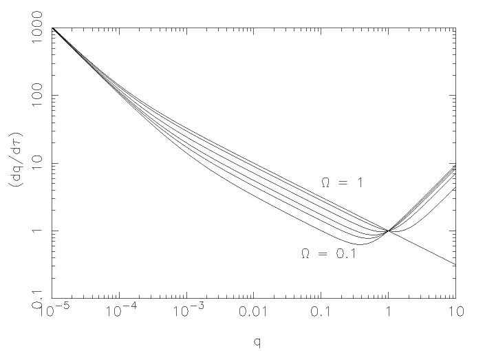Figure 2. The phase portrait of the universe, with the "velocity" of the universe (dq / d) plotted against the "position" q = (1 + z)-1 for different models with R = 2.56 × 10-5h-2, h = 0.5, NR + + R = 1. Curves are parameterized by the value of NR = 0.1, 0.2, 0.3, 0.5, 0.8, 1.0 going from bottom to top as indicated. (Figure adapted from [46].)

For a universe with non relativistic matter and cosmological constant, the potential in (25) has a simple form, varying as (- a^-1) for small a and (- a²) for large a with a maximum in between at q = q_max = (_NR / 2)^1/3. This system has been analyzed in detail in literature for both constant cosmological constant [67] and for a time dependent cosmological constant [68]. A wide variety of explicit solutions for a(t) can be provided for these equations. We briefly summarize a few of them.

• If the "particle" is situated at the top of the potential, one can obtain a static solution with = = 0 by adjusting the cosmological constant and the dust energy density and taking k = 1. This solution,

  (26)

  was the one which originally prompted Einstein to introduce the cosmological constant (see section 1.2).

• The above solution is, obviously, unstable and any small deviation from the equilibrium position will cause a 0 or a . By fine tuning the values, it is possible to obtain a model for the universe which "loiters" around a = a_max for a large period of time [69, 70, 71, 24, 25, 26].
• A subset of models corresponds to those without matter and driven entirely by cosmological constant . These models have k = (- 1, 0, + 1) and the corresponding expansion factors being proportional to [sinh(Ht), exp(Ht), cosh(Ht)] with ² = 3H². These line elements represent three different characterizations of the de Sitter spacetime. The manifold is a four dimensional hyperboloid embedded in a flat, five dimensional space with signature (+ - - -). We shall discuss this in greater detail in section 9.
• It is also possible to obtain solutions in which the particle starts from a = 0 with an energy which is insufficient for it to overcome the potential barrier. These models lead to a universe which collapses back to a singularity. By arranging the parameters suitably, it is possible to make a(t) move away or towards the peak of the potential (which corresponds to the static Einstien universe) asymptotically [67].
• In the case of _NR + = 1, the explicit solution for a(t) is given by

  (27)

  This solution smoothly interpolates between a matter dominated universe a(t) t^2/3 at early stages and a cosmological constant dominated phase a(t) exp(Ht) at late stages. The transition from deceleration to acceleration occurs at z_acc = (2 / _NR)^1/3 - 1, while the energy densities of the cosmological constant and the matter are equal at z_m = ( / _NR)^1/3 - 1.

The presence of a cosmological constant also affects other geometrical parameters in the universe. Figure 3 gives the plot of d_A(z) and d_L(z); (note that angular diameter distance is not a monotonic function of z). Asymptotically, for large z, these have the limiting forms,

(28)

Figure 3. The left panel gives the angular diameter distance in units of cH0-1 as a function of redshift. The right panel gives the luminosity distance in units of cH0-1 as a function of redshift. Each curve is labelled by (NR, ).

The geometry of the spacetime also determines the proper volume of the universe between the redshifts z and z + dz which subtends a solid angle d in the sky. If the number density of sources of a particular kind (say, galaxies, quasars, ...) is given by n(z), then the number count of sources per unit solid angle per redshift interval should vary as

(29)

Figure 4 shows (dN / ddz); it is assumed that n(z) = n₀(1 + z)³. The y-axis is in units of n₀ H₀^-3.

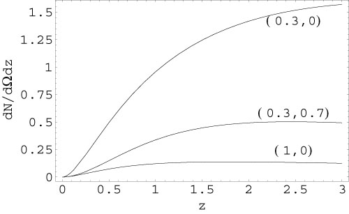Figure 4. The figure shows (dN / ddz): it is assumed that n(z) = n0(1 + z)3. The y-axis is in units of n0H0-3. Each curve is labelled by (NR, ).