


There are several cosmological observations which suggests the existence of
a non zero cosmological constant with different levels of reliability.
Most of these determine either the value of
 NR
or some combination of
NR and
NR
or some combination of
NR and
 .
When combined with the strong evidence from the CMBR observations that
the tot = 1
(see section 6) or some other independent
estimate of
NR,
one is led to a non zero value for
.
The most reliable ones seem to be those based on high redshift supernova
[72,
73,
74]
and structure formation models
[75,
76,
77].
We shall now discuss some of these evidence.
.
When combined with the strong evidence from the CMBR observations that
the tot = 1
(see section 6) or some other independent
estimate of
NR,
one is led to a non zero value for
.
The most reliable ones seem to be those based on high redshift supernova
[72,
73,
74]
and structure formation models
[75,
76,
77].
We shall now discuss some of these evidence.
3.1. Observational evidence for accelerating universe
Figure 2 shows that the evolution of
a universe with
 0
changes from a decelerating phase to an accelerating phase at late times.
If H(a) can be observationally determined, then one can check
whether the real universe had undergone an accelerating phase
in the past. This, in turn, can be done if
dL(z), say, can be observationally
determined for a class of sources. Such a study of several high redshift
supernova has led to the data which is shown in
figures 5, 9.
0
changes from a decelerating phase to an accelerating phase at late times.
If H(a) can be observationally determined, then one can check
whether the real universe had undergone an accelerating phase
in the past. This, in turn, can be done if
dL(z), say, can be observationally
determined for a class of sources. Such a study of several high redshift
supernova has led to the data which is shown in
figures 5, 9.
Bright supernova explosions are brief events (~ 1 month) and occurs in our galaxy typically once in 300 years. These are broadly classified as two types. Type-Ia supernova occurs when a degenerate dwarf star containing CNO enters a stage of rapid nuclear burning cooking iron group elements (see eg., chapter 7 of [78]). These are the brightest and most homogeneous class of supernova with hydrogen poor spectra. An empirical correlation has been observed between the sharply rising light curve in the initial phase of the supernova and its peak luminosity so that they can serve as standard candles. (Type II supernova, which occur at the end of stellar evolution, are not useful for this purpose.)
For any supernova, one can directly observe the apparent magnitude m
[which is essentially the logarithm of the flux F observed]
and its redshift. The absolute magnitude M of the supernova is
again related to the actual luminosity L of the supernova
in a logarithmic fashion. Hence the relation
F = (L / 4 dL2) can be written as
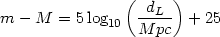 |
(30) |
The numerical factors arise from the astronomical conventions used in
the definition of m and M. Very often,
one will use the dimensionless combination
(H0 dL(z) / c) rather
than dL(z) and the above equation
will change to
m(z) =  + 5 log10 Q(z).
The results below will be often stated in terms of the quantity
, related to M by
+ 5 log10 Q(z).
The results below will be often stated in terms of the quantity
, related to M by
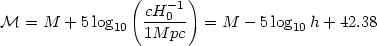 |
(31) |
If the absolute magnitude of a class of Type I supernova can be determined from the study of its light curve, then one can obtain the dL for these supernova at different redshifts. Knowing dL, one can determine the geometry of the universe.
To understand this effect in a simple context, let us compare
the luminosity distance for a matter dominated model
(NR = 1,
= 0)
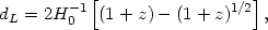 |
(32) |
with that for a model driven purely by a cosmological constant
(NR = 0,
= 1):
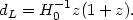 |
(33) |
It is clear that at a given z, the dL is larger for the cosmological constant model. Hence, a given object, located at a fixed redshift, will appear brighter in the matter dominated model compared to the cosmological constant dominated model. Though this sounds easy in principle, the statistical analysis turns out to be quite complicated.
The high-z supernova search team (HSST) discovered about 16 supernova
in the redshift range (0.16 - 0.62) and another 34 nearby supernova
[73] and used
two separate methods for data fitting.
The supernova cosmology project (SCP) has discovered
[74]
42 supernova in the range (0.18 - 0.83). Assuming
NR +
=
1, the analysis of this data gives
NR = 0.28
± 0.085 (stat) ± 0.05 (syst).
Figure 5 shows the
dL(z) obtained from the supernova data and
three theoretical curves
all of which are for k = 0 models containing non relativistic
matter and cosmological constant.
The data used here is based on the redshift magnitude relation of 54
supernova (excluding
6 outliers from a full sample of 60) and that of SN 1997ff at z =
1.755; the magnitude used
for SN 1997ff has been corrected for lensing effects.
The best fit curve has
NR
 0.32,
0.68. In this analysis,
one had treated
NR and
the absolute magnitude M as free parameters (with
NR +
= 1)
and has done a simple best fit for both.
The corresponding best fit value for
is
= 23.92 ± 0.05.
Frame (a) of figure 6 shows the confidence
interval (for 68 %, 90 % and 99 %) in the
NR -
for the flat
models. It is obvious that
most of the probability is concentrated around the best fit value.
We shall discuss frame (b) and frame (c) later on.
(The discussion here is based on
[79].)
0.32,
0.68. In this analysis,
one had treated
NR and
the absolute magnitude M as free parameters (with
NR +
= 1)
and has done a simple best fit for both.
The corresponding best fit value for
is
= 23.92 ± 0.05.
Frame (a) of figure 6 shows the confidence
interval (for 68 %, 90 % and 99 %) in the
NR -
for the flat
models. It is obvious that
most of the probability is concentrated around the best fit value.
We shall discuss frame (b) and frame (c) later on.
(The discussion here is based on
[79].)
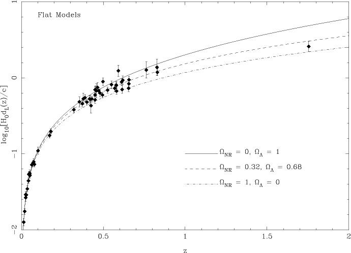 |
Figure 5. The luminosity distance
of a set of type Ia supernova at different redshifts and three
theoretical models with
|
 |
Figure 6. Confidence contours corresponding
to 68 %, 90 % and 99 % based on SN data in the
|
The confidence intervals in the
-
NR plane are
shown in figure 7 for the full data. The
confidence regions in the top left frame are obtained
after marginalizing over
. (The best fit value
with 1 error is
indicated in each panel and the confidence contours correspond to 68 %,
90 % and 99 %.) The other three frames show the corresponding result
with a constant value for
rather than by
marginalizing over this parameter. The three frames
correspond to the mean value and two values in the wings of
1 from the mean.
The dashed line connecting the points (0,1) and (1,0) correspond to a
universe with
NR +
= 1.
From the figure we can conclude that: (i) The results do not change
significantly whether we marginalize over
or whether we use the
best fit value. This is a direct consequence of the result in frame (a) of
figure (6) which
shows that the probability is sharply peaked. (ii) The results exclude
the NR = 1,
= 0 model at a
high level of significance in spite of the uncertainty in
.
error is
indicated in each panel and the confidence contours correspond to 68 %,
90 % and 99 %.) The other three frames show the corresponding result
with a constant value for
rather than by
marginalizing over this parameter. The three frames
correspond to the mean value and two values in the wings of
1 from the mean.
The dashed line connecting the points (0,1) and (1,0) correspond to a
universe with
NR +
= 1.
From the figure we can conclude that: (i) The results do not change
significantly whether we marginalize over
or whether we use the
best fit value. This is a direct consequence of the result in frame (a) of
figure (6) which
shows that the probability is sharply peaked. (ii) The results exclude
the NR = 1,
= 0 model at a
high level of significance in spite of the uncertainty in
.
 |
Figure 7. Confidence contours corresponding
to 68 %, 90 % and 99 % based on SN data in the
|
The slanted shape of the probability ellipses shows that a particular
linear combination of
NR and
is
selected out by these observations
[80].
This feature, of course, has nothing to do with supernova and arises purely
because the luminosity distance dL depends strongly on
a particular linear combination of
and
NR, as
illustrated in figure 8.
In this figure,
NR,
are treated as free parameters [without the k = 0 constraint]
but a particular linear combination
q  (0.8NR -
0.6) is held
fixed. The dL is not very sensitive to
individual values of
NR,
at low redshifts
when
(0.8NR -
0.6) is in the range
of (- 0.3, - 0.1). Though some of the models have unacceptable parameter
values (for other reasons), supernova measurements alone cannot rule
them out. Essentially the data at
z < 1 is degenerate on the linear combination of parameters
used to construct the variable q. The supernova data shows that
most likely region is bounded by
-0.3
(0.8NR -
0.6) is held
fixed. The dL is not very sensitive to
individual values of
NR,
at low redshifts
when
(0.8NR -
0.6) is in the range
of (- 0.3, - 0.1). Though some of the models have unacceptable parameter
values (for other reasons), supernova measurements alone cannot rule
them out. Essentially the data at
z < 1 is degenerate on the linear combination of parameters
used to construct the variable q. The supernova data shows that
most likely region is bounded by
-0.3  (0.8NR -
0.6)
- 0.1.
In figure 7 we have also over plotted the line
corresponding to
H0 dL(z = 0.63) =
constant. The coincidence of this line (which roughly corresponds to
dL at a redshift in the middle of the data) with the
probability ellipses indicates that it is this quantity which
essentially determines the nature of the result.
(0.8NR -
0.6)
- 0.1.
In figure 7 we have also over plotted the line
corresponding to
H0 dL(z = 0.63) =
constant. The coincidence of this line (which roughly corresponds to
dL at a redshift in the middle of the data) with the
probability ellipses indicates that it is this quantity which
essentially determines the nature of the result.
 |
Figure 8. The luminosity distance for a
class of models with widely varying
|
We saw earlier that the presence of cosmological constant leads to an
accelerating phase in the universe
which - however - is not obvious from the above figures.
To see this explicitly one needs to display the data in the
 vs a plane, which is done in
figure 9.
Direct observations of supernova is converted into
dL(z) keeping
M a free parameter. The dL is converted into
dH(z)
assuming k = 0 and using (17). A best fit analysis, keeping
(M,
NR)
as free parameters now lead to the results shown in
figure 9, which
confirms the accelerating phase in the evolution of the universe.
The curves which are over-plotted correspond to a cosmological model
with
NR +
= 1. The best
fit curve has
NR =
0.32,
= 0.68.
vs a plane, which is done in
figure 9.
Direct observations of supernova is converted into
dL(z) keeping
M a free parameter. The dL is converted into
dH(z)
assuming k = 0 and using (17). A best fit analysis, keeping
(M,
NR)
as free parameters now lead to the results shown in
figure 9, which
confirms the accelerating phase in the evolution of the universe.
The curves which are over-plotted correspond to a cosmological model
with
NR +
= 1. The best
fit curve has
NR =
0.32,
= 0.68.
 |
Figure 9. Observations of SN are converted
into the `velocity' |
In the presence of the cosmological constant, the universe accelerates
at low redshifts while
decelerating at high redshift. Hence, in principle, low redshift
supernova data should indicate the evidence for acceleration. In
practice, however, it is impossible to rule out any of the cosmological
models using low redshift
(z 0.2)
data as is evident from figure 9.
On the other hand, high redshift supernova data alone cannot be
used to establish the existence of a cosmological constant. The data for
(z  0.2) in
figure 9 can be moved vertically up and made
consistent with the decelerating
= 1 universe by
choosing the absolute magnitude M suitably. It is the interplay
between both the high
redshift and low redshift supernova which leads to the result quoted above.
0.2) in
figure 9 can be moved vertically up and made
consistent with the decelerating
= 1 universe by
choosing the absolute magnitude M suitably. It is the interplay
between both the high
redshift and low redshift supernova which leads to the result quoted above.
This important result can be brought out more quantitatively along the
following lines. The data displayed in figure 9
divides the supernova into two natural classes: low redshift ones in the
range 0 < z
0.25
(corresponding to the accelerating phase of the universe)
and the high redshift ones in the range
0.25 z
2 (in the
decelerating phase of the universe).
One can repeat all the statistical analysis for the full set as well as
for the two
individual low redshift and high redshift data sets. Frame (b) and (c)
of figure 6 shows the confidence interval based
on low redshift
data and high redshift data separately. It is obvious that the
NR = 1 model
cannot be ruled out with either of the two data sets!
But, when the data sets are combined - because of the angular slant of the
ellipses - they isolate a best fit region around
NR
0.3.
This is also seen in figure 10 which plots the
confidence intervals using just the high-z and low-z data
separately. The right most frame in the bottom row is based on the low-z
data alone (with marginalisation over
) and this data cannot
be used to discriminate between cosmological models effectively. This is
because the dL at low-z is only very weakly dependent
on the cosmological parameters. So, even though the acceleration of the
universe is a low-z phenomenon, we cannot reliably determine it using
low-z data alone. The top left frame has the corresponding result with
high-z data. As we stressed before, the
NR = 1
model cannot be excluded on the basis of the high-z data alone
either. This is essentially because of the nature of probability
contours seen earlier in frame (c) of
figure 6. The remaining 3 frames (top right,
bottom left and bottom middle) show the corresponding results in which
fixed values of
- rather than by
marginalising over
. Comparing these
three figures with the corresponding three frames in
7 in which all
data was used, one can draw the following conclusions: (i) The best fit
value for
is now
= 24.05 ± 0.38;
the 1 error has now
gone up by nearly eight times compared to the result (0.05) obtained
using all data.
Because of this spread, the results are sensitive to the value of
that one uses,
unlike the situation in which all data was used. (ii) Our conclusions
will now depend on
.
For the mean value and lower end of
, the data can exclude
the NR = 1,
= 0 model
[see the two middle frames of figure 10].
But, for the high-end of allowed
1 range of
, we cannot exclude the
NR = 1,
= 0 model [see
the bottom left frame of figure 10].
 |
Figure 10. Confidence contours
corresponding to 68 %, 90 % and 99 % based on SN data in the
|
While these observations have enjoyed significant popularity, certain key points which underly these analysis need to be stressed. (For a sample of views which goes against the main stream, see [81, 82]).
NR,
V)
(0.8, 1.5)
which is strongly disfavoured by several other observations.
If this disparity is due to some other unknown systematic
effect, then this will have an effect on the estimate given above.
NR which
is consistent with unity:
NR =
(0.94+0.34-0.28). However, adding a single
z = 0.83 supernova for which good HST data was available, lowered the
value to
NR = (0.6
± 0.2). More recently, the analysis
of a larger data set of 42 high redshift SNe Ia gives the results quoted
above.