5.1. Linear evolution of perturbations

When the perturbations are small, one can ignore the second term in the right hand side of (65) and replace (1 + ) by unity in the first term on the right hand side. The resulting equation is valid in the linear regime and hence will be satisfied by each of the Fourier modes _k(t) obtained by Fourier transforming (t, x) with respect to x. Taking (t, x) = D(t) f (x), the D(t) satisfies the equation

(66)

The power spectra P(k, t) = < |_k(t)|² > at two different redshifts in the linear regime are related by

(67)

where T (called transfer function) depends only on the parameters of the background universe (denoted by `bg') but not on the initial power spectrum and can be computed by solving (66). It is now clear that the only new input which structure formation scenarios require is the specification of the initial perturbation at all relevant scales, which requires one arbitrary function of the wavenumber k = 2 / .

Let us first consider the transfer function. The rate of growth of small perturbations is essentially decided by two factors: (i) The relative magnitudes of the proper wavelength of perturbation _prop(t) a(t) and the Hubble radius d_H(t) H^-1(t) = ( / a)^-1 and (ii) whether the universe is radiation dominated or matter dominated. At sufficiently early epochs, the universe will be radiation dominated and d_H(t) t will be smaller than the proper wavelength _prop(t) t^1/2. The density contrast of such modes, which are bigger than the Hubble radius, will grow as a² until _prop = d_H(t). [When this occurs, the perturbation at a given wavelength is said to enter the Hubble radius. One can use (66) with the right hand side replaced by 4(1 + w)(1 + 3w) G in this case; this leads to D t a².] When _prop < d_H and the universe is radiation dominated, the perturbation does not grow significantly and increases at best only logarithmically [193]. Later on, when the universe becomes matter dominated for t > t_eq, the perturbations again begin to grow. It follows from this result that modes with wavelengths greater than d_eq d_H(t_eq) - which enter the Hubble radius only in the matter dominated epoch - continue to grow at all times while modes with wavelengths smaller than d_eq suffer lack of growth (in comparison with longer wavelength modes) during the period t_enter < t < t_eq. This fact leads to a distortion of the shape of the primordial spectrum by suppressing the growth of small wavelength modes in comparison with longer ones. Very roughly, the shape of T²(k) can be characterized by the behaviour T²(k) k^-4 for k > k_eq and T² 1 for k < k_eq. The wave number k_eq corresponds to the length scale

(68)

(eg., [44], p.75). The spectrum at wavelengths >> d_eq is undistorted by the evolution since T² is essentially unity at these scales. Further evolution can eventually lead to nonlinear structures seen today in the universe.

At late times, we can ignore the effect of radiation in solving (66). The linear perturbation equation (66) has an exact solution (in terms of hyper-geometric functions) for cosmological models with non-relativistic matter and dark energy with a constant w. It is given by

(69)

Figure 15 shows the growth factor for different values of w including the one for cosmological constant (corresponding to w = - 1) and an open model (with w = -1/3.)

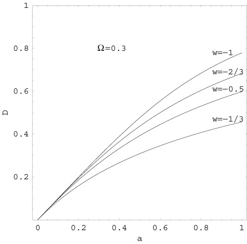Figure 15. The growth factor for different values of w including the one for cosmological constant (corresponding to w = - 1) and an open model (with w = - 1/3).

For small values of a, D a which is an exact result for = 0, _NR = 1 model. The growth rate slows down in the cosmological constant dominated phase (in models with _NR + = 1 with w = - 1) or in the curvature dominated phase (open models with _NR < 1 corresponding to w = - 1/3). Between the two cases, there is less growth in open models compared to models with cosmological constant.

It is possible to rewrite equation (65) in a different form to find an approximate solution for even variable w(a). Converting the time derivatives into derivatives with respect to a (denoted by a prime) and using the Friedmann equations, we can write (65) as

(70)

In a universe populated by only non relativistic matter and dark energy characterized by an equation of state function w(a), this equation can be recast in a different manner by introducing a time dependent [as in equation (43)] by the relation Q(t) = (8 G / 3) [_NR(t) / H²(t)] so that (dQ/d ln a) = 3wQ(1 - Q). Then equation (65) becomes in terms of the variable f (d ln / d ln a)

(71)

Unfortunately this equation is not closed in terms of f and Q since it also involves = exp[(da / a)f]. But in the linear regime, we can ignore the second term on the right hand side and replace (1 + ) by unity in the first term thereby getting a closed equation:

(72)

This equation has approximate power law solutions [189] of the form f = Qⁿ when |dw / dQ| << 1 / (1 - Q). Substituting this ansatz, we get

(73)

[Note that Q(t) 1 at high redshifts, which is anyway the domain of validity of the linear perturbation theory]. This result shows that n is weakly dependent on _NR; further, n (4/7) for open Friedmann model with non relativistic matter and n (6/11) 0.6 in a k = 0 model with cosmological constant.

It is possible to provide simple analytic fitting functions for the transfer function, incorporating all the above effects. For models with a cosmological constant, the transfer function is well fitted by [194]

(74)

where p = k / ( h Mpc^-1) and = _NR h exp[- _B(1 + (2 h)^1/2 / _NR)] is called the `shape factor'.

Let us next consider the initial power spectrum P(k, z_i). The following points need to be emphasized regarding the initial fluctuation spectrum.

(1) It can be proved that known local physical phenomena, arising from laws tested in the laboratory in a medium with (P/) > 0, are incapable producing the initial fluctuations of required magnitude and spectrum (eg., [9], p. 458). The initial fluctuations, therefore, must be treated as arising from physics untested at the moment.

(2) Contrary to claims sometimes made in the literature, inflationary models are not capable of uniquely predicting the initial fluctuations. It is possible to come up with viable inflationary potentials ([196], chapter 3) which are capable of producing any reasonable initial fluctuation.

A prediction of the initial fluctuation spectrum was indeed made by Harrison [197] and Zeldovich [198], who were years ahead of their times. They predicted - based on very general arguments of scale invariance - that the initial fluctuations will have a power spectrum P = Akⁿ with n = 1. Considering the simplicity and importance of this result, we shall briefly recall the arguments leading to the choice of n = 1.

If the power spectrum is P kⁿ at some early epoch, then the power per logarithmic band of wave numbers is ² k³P(k) k⁽ⁿ⁺³⁾. Further, when the wavelength of the mode is larger than the Hubble radius, d_H(t) = ( / a)^-1, during the radiation dominated phase, the perturbation grows as a² making ² a⁴k⁽ⁿ⁺³⁾. We need to determine how scales with k when the mode enters the Hubble radius d_H(t). The epoch a_enter at which this occurs is determined by the relation 2 a_enter / k = d_H. Using d_H t a² in the radiation dominated phase, we get a_enter k^-1 so that

(75)

It follows that the amplitude of fluctuations is independent of scale k at the time of entering the Hubble radius, only if n = 1. This is the essence of Harrison-Zeldovich and which is independent of the inflationary paradigm. It follows that verification of n = 1 by any observation is not a verification of inflation. At best it verifies a far deeper principle of scale invariance. We also note that the power spectrum of gravitational potential P scales as P P / k⁴ k^(n-4). Hence the fluctuation in the gravitational potential (per decade in k) ² k³ P is proportional to ² k^(n-1). This fluctuation in the gravitational potential is also independent of k for n = 1 clearly showing the special nature of this choice.[It is not possible to take n strictly equal to unity without specifying a detailed model; the reason has to do with the fact that scale invariance is always broken at some level and this will lead to a small difference between n and unity]. Given the above description, the basic model of cosmology is based on seven parameters. Of these 5 parameters (H₀, _B, _DM, , _R) determine the background universe and the two parameters (A, n) specify the initial fluctuation spectrum.

The presence of dark energy, with a constant w, will also affect the transfer function and hence the final power spectrum. An approximate fitting formula can be given along the following lines [195]. Let the power spectrum be written in the form

(76)

where A_Q is a normalization, T_Q is the modified transfer function and g_Q = (D / a) is the ratio between linear growth factor in the presence of dark energy compared to that in = 1 model. Writing T_Q as the product T_Q T where T is given by (74), numerical work shows that

(77)

where k is in Mpc^-1, and is a scale-independent but time-dependent coefficient well approximated by = (-w)^s with

(78)

where the matter density parameter is _NR(a) = _NR / [_NR + (1 - _NR) a^-3w]. Similarly, the relative growth factor can be expressed in the form g_Q (g_Q / g) = (- w)^t with

(79)

Finally the amplitude A_Q can be expressed in the form A_Q = _H²(c / H₀)ⁿ⁺³ / (4), where

(80)

and ₀ = (a = 1) of equation (78), and

(81)

This fit is valid for -1 w - 0.2.