6. CMBR ANISOTROPIES

In the standard Friedmann model of the universe, neutral atomic systems form at a redshift of about z 10³ and the photons decouple from the matter at this redshift. These photons, propagating freely in spacetime since then, constitute the CMBR observed around us today. In an ideal Friedmann universe, for a comoving observer, this radiation will appear to be isotropic. But if physical process has led to inhomogeneities in the z = 10³ spatial surface, then these inhomogeneities will appear as angular anisotropies in the CMBR in the sky today. A physical process operating at a proper length scale L on the z = 10³ surface will lead to an effect at an angle = L / d_A(z). Numerically,

(95)

To relate the theoretical predictions to observations, it is usual to expand the temperature anisotropies in the sky in terms of the spherical harmonics. The temperature anisotropy in the sky will provide = T / T as a function of two angles and . If we expand the temperature anisotropy distribution on the sky in spherical harmonics:

(96)

all the information is now contained in the angular coefficients a_lm.

If n and m are two directions in the sky with an angle between them, the two-point correlation function of the temperature fluctuations in the sky can be defined as

(97)

Since the sources of temperature fluctuations are related linearly to the density inhomogeneities, the coefficients a_lm will be random fields with some power spectrum. In that case < a_lma^*_l'm' > will be nonzero only if l = l' and m = m'. Writing

(98)

and using the addition theorem of spherical harmonics, we find that

(99)

with C_l = < | a_lm|² >. In this approach, the pattern of anisotropy is contained in the variation of C_l with l. Roughly speaking, l ^-1 and we can think of the (, l ) pair as analogue of (x, k) variables in 3-D. The C_l is similar to the power spectrum P(k).

In the simplest scenario, the primary anisotropies of the CMBR arise from three different sources. (i) The first is the gravitational potential fluctuations at the last scattering surface (LSS) which will contribute an anisotropy (T / T)² k³ P(k) where P(k) P(k) / k⁴ is the power spectrum of gravitational potential . This anisotropy arises because photons climbing out of deeper gravitational wells lose more energy on the average. (ii) The second source is the Doppler shift of the frequency of the photons when they are last scattered by moving electrons on the LSS. This is proportional to ( T / T)_D² k³ P_v where P_v(k) P / k² is the power spectrum of the velocity field. (iii) Finally, we also need to take into account the intrinsic fluctuations of the radiation field on the LSS. In the case of adiabatic fluctuations, these will be proportional to the density fluctuations of matter on the LSS and hence will vary as ( T / T)_int² k³ P(k). Of these, the velocity field and the density field (leading to the Doppler anisotropy and intrinsic anisotropy described in (ii) and (iii) above) will oscillate at scales smaller than the Hubble radius at the time of decoupling since pressure support will be effective at these scales. At large scales, if P(k) k, then

(100)

where k^-1 is the angular scale over which the anisotropy is measured. Obviously, the fluctuations due to gravitational potential dominate at large scales while the sum of intrinsic and Doppler anisotropies will dominate at small scales. Since the latter two are oscillatory, we sill expect an oscillatory behaviour in the temperature anisotropies at small angular scales.

There is, however, one more feature which we need to take into account. The above analysis is valid if recombination was instantaneous; but in reality the thickness of the recombination epoch is about z 80 ([220]; [44], chapter 3). This implies that the anisotropies will be damped at scales smaller than the length scale corresponding to a redshift interval of z = 80. The typical value for the peaks of the oscillation are at about 0.3 to 0.5 degrees depending on the details of the model. At angular scales smaller than about 0.1 degree, the anisotropies are heavily damped by the thickness of the LSS.

The fact that several different processes contribute to the structure of angular anisotropies make CMBR a valuable tool for extracting cosmological information. To begin with, the anisotropy at very large scales directly probe modes which are bigger than the Hubble radius at the time of decoupling and allows us to directly determine the primordial spectrum. Thus, in general, if the angular dependence of the spectrum at very large scales is known, one can work backwards and determine the initial power spectrum. If the initial power spectrum is assumed to be P(k) = Ak, then the observations of large angle anisotropy allows us to fix the amplitude A of the power spectrum [207, 208]. Based on the results of COBE satellite [221], one finds that the amount of initial power per logarithmic band in k space is given by

(101)

This corresponds to A (28.6h^-1 Mpc)⁴ and an initial fluctuation in the gravitational potential of 3.1 × 10^-5. This result is powerful enough to rule out matter dominated, = 1 models when combined with the data on the abundance of large clusters which determines the amplitude of the power spectrum at R 8h^-1 Mpc. For example the parameter values h = 0.5, _{0 DM} = 1, = 0, are ruled out by this observation when combined with COBE observations [207, 208].

As we move to smaller scales we are probing the behaviour of baryonic gas coupled to the photons. The pressure support of the gas leads to modulated acoustic oscillations with a characteristic wavelength at the z = 10³ surface. Regions of high and low baryonic density contrast will lead to anisotropies in the temperature with the same characteristic wavelength. The physics of these oscillations has been studied in several papers in detail [222, 223, 224, 225, 226, 227, 228, 229, 230]. The angle subtended by the wavelength of these acoustic oscillations will lead to a series of peaks in the temperature anisotropy which has been detected [231, 232]. The structure of acoustic peaks at small scales provides a reliable procedure for estimating the cosmological parameters.

To illustrate this point let us consider the location of the first acoustic peak. Since all the Fourier components of the growing density perturbation start with zero amplitude at high redshift, the condition for a mode with a given wave vector k to reach an extremum amplitude at t = t_dec is given by

(102)

where c_s = (P / )^1/2 (1 / 3) is the speed of sound in the baryon-photon fluid. At high redshifts, t(z) _NR^-1/2(1 + z)^-3/2 and the proper wavelength of the first acoustic peak scales as _peak ~ t_dec h^-1 _NR^-1/2. The angle subtended by this scale in the sky depends on d_A. If _NR + = 1 then the angular diameter distance varies as _NR^-0.4 while if = 0, it varies as _NR^-1. It follows that the angular size of the acoustic peak varies with the matter density as

(103)

Therefore, the angle subtended by acoustic peak is quite sensitive to _NR if = 0 but not if _NR + = 1. More detailed computations show that the multipole index corresponding to the acoustic peak scales as l_p 220 _NR^-1/2 if = 0 and l_p 220 if _NR + = 1 and 0.1 _NR 1. This is illustrated in figure 17 which shows the variation in the structure of acoustic peaks when is changed keeping = 0. The four curves are for = _NR = 0.25, 0.45, 1.0, 1.15 with the first acoustic peak moving from right to left. The data points on the figures are from the first results of MAXIMA and BOOMERANG experiments and are included to give a feel for the error bars in current observations. It is obvious that the overall geometry of the universe can be easily fixed by the study of CMBR anisotropy.

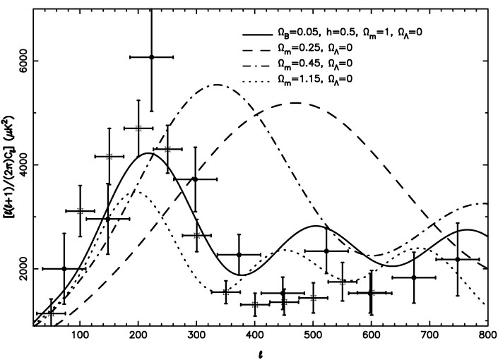Figure 17. The variation of the anisotropy pattern in universes with NR = (0.25, 0.45, 1.0, 1.15), = 0 with the first acoustic peak moving from right to left. The y-axis is essentially a measure of ( T / T)2 while the x-axis is a measure of 1/.( Figure courtesy: S.Sethi.)

At present there exists several observations of the small scale anisotropies in the CMBR from the balloon flights, BOOMERANG [231], MAXIMA [232], and from radio telescopes CBI [233], VSA [234], and DASI [235, 236]. These CMBR data has been extensively analyzed in isolation as well as in combination with other results [59, 60, 221, 233, 234, 237, 238, 239, 240, 241, 242]. (The information about structure formation arises mainly from galaxy surveys like SSRS2, CfA2 [243], LCRS [244], Abell-ACO cluster survey [245], IRAS-PSC z [240] and the 2-D survey [246, 239].) While there is some amount of variations in the results, by and large, they support the following conclusions.

• The data strongly supports a k = 0 model of the universe [242] with _tot = 1.00 ± ^0.03_0.02.
• Combined with large scale structure data, the results suggest _NR = 0.29 ± 0.05 ± 0.04 [59, 60, 242, 247]. The initial power spectrum is consistent with being scale invariant and n = 1.02 ± 0.06 ± 0.05 [59, 60, 242]. In fact, combining 2dF survey results with CMBR suggest [248] 0.7 independent of the supernova results.
• A similar analysis based on BOOMERANG data leads to _tot = 1.02 ± 0.06(see for example, [238]). Combining this result with the HST constraint [49] on the Hubble constant h = 0.72 ± 0.08, galaxy clustering data as well SN observations one gets = 0.62^0.10_-0.18, = 0.55^0.09_-0.09 and = 0.73^0.10_-0.07 respectively [249].
• The analysis also gives an independent handle on baryonic density in the universe which is consistent with the BBN value: _B h² = 0.022 ± 0.003 [59, 60]. This is gratifying since the initial data had an error and gave too high a value [250].

There has been some amount of work on the effect of dark energy on the CMBR anisotropy [251, 252, 253, 254, 255, 256, 257]. The shape of the CMB spectrum is relatively insensitive to the dark energy and the main effect is to alter the angular diameter distance to the last scattering surface and thus the position of the first acoustic peak. Several studies have attempted to put a bound on w using the CMB observations. Depending on the assumptions which were invoked, they all lead to a bound broadly in the range of w - 0.6. At present it is not clear whether CMBR anisotropies can be of significant help in discriminating between different dark energy models.