5.5. Inverse cascades

A relevant topic in the evolution of large scale magnetic fields concerns the concepts of direct and inverse cascades. A direct cascade is a process, occurring in a plasma, where energy is transferred from large to small length scales. An inverse cascade is a process where the energy transfer goes from small scales to large length scales. One can also generalize the the concept of energy cascade to the cascade of any conserved quantity in the plasma, like, for instance, the helicity. Thus, in general terms, the transfer process of a conserved quantity is a cascade.

The concept of cascade (either direct or inverse) is related with the concept of turbulence, i.e. the class of phenomena taking place in fluids and plasmas at high Reynolds numbers, as anticipated in Section 4. Non-magnetized fluids become turbulent at high kinetic Reynolds numbers. Similarly, magnetized fluids should become turbulent for sufficiently large magnetic Reynolds numbers. The experimental evidence of this occurrence is still poor. One of the reasons is that it is very difficult to reach, with terrestrial plasmas, the physical situation where the magnetic and the kinetic Reynolds numbers are both large but, in such a way that their ratio is also large i.e.

(5.93)

The physical regime expressed through Eqs. (5.93) rather common in the early Universe. Thus, MHD turbulence is probably one of the key aspects of magnetized plasma dynamics at very high temperatures and densities. Consider, for instance, the plasma at the electroweak epoch when the temperature was of the order of 100 GeV. One can compute the Reynolds numbers and the Prandtl number from their definitions given in Eqs. (4.40)-(4.42). In particular,

(5.94)

which can be obtained from Eqs. (4.40)-(4.42) using as fiducial parameters v 0.1, T / , (T)^-1 and L 0.01 H_ew^-1 0.03 cm for T 100 GeV.

At high Reynolds and Prandtl numbers the evolution of the large-scale magnetic fields is not obvious since the inertial regime is large. There are then two scales separated by a huge gap: the scale of the horizon (3 cm at the electroweak epoch) and the diffusivity scale (about 10^-8 cm). One would like to know, given an initial spectrum of the magnetic fields, what is the evolution of the spectrum, i.e. in what modes the energy has been transferred. The problem is that it is difficult to simulate systems with huge hierarchies of scales.

Suppose, for instance, that large scale magnetic fields are generated at some time t₀ and with a given spectral dependence. The energy spectrum of magnetic fields may receive, for instance, the dominant contribution for large comoving momentum k (close to the cut-off provided by the magnetic diffusivity scale). The "initial" spectrum at the time t₀ is sometimes called injection spectrum. The problem will then be to know the how the spectrum is modified at a later time t. If inverse cascade occurs, the magnetic energy density present in the ultra-violet modes may be transferred to the infra-red modes. In spite of the fact that inverse cascades are a powerful dynamical principle, it is debatable under which conditions they may arise.

The possible occurrence of inverse cascades in a magnetized Universe has been put forward, in a series of papers, by Brandenburg, Enqvist and Olesen [145, 146, 147, 148] (see also [149] for an excellent review covering also in a concise way different mechanisms for the generation of large-scale magnetic fields).

MHD simulations in 2 + 1 dimensions [145, 146] seem to support the idea of an inverse cascade in a radiation dominated Universe. Two-dimensional MHD simulations are very interesting but also peculiar. In 2 + 1 dimensions, the magnetic helicity does not exist while the magnetic flux is well defined and conserved in the ideal MHD limit. It is therefore impossible to implement 2 + 1-dimensional MHD simulations where the magnetic flux and the magnetic helicity are constrained to be constant in the ideal limit. This technical problem is related to a deeper physical difference between magnetized plasmas with and without helicity. Consider then, for the moment, the situation where the helicity is strictly zero. It is indeed possible to argue that, in this case, 2 + 1-dimensional MHD simulations can capture some of the relevant features of 3 + 1-dimensional MHD evolution.

In [147, 148] the scaling properties of MHD equations have been investigated in the force-free regime (i.e. in the approximation of negligible Lorentz force). In the absence of helical components at the onset of the MHD evolution a rather simple argument has been proposed by Olesen [147] in order to decide under which conditions inverse cascade may arise. Consider the magnetic diffusivity and Navier-Stokes equations in the limit where × 0. Then, the evolution equations are invariant under the following similarity transformations:

(5.95)

For simplicity it is also useful to concentrate the attention on the inertial range of momenta where the dynamics is independent on the scale of dissipation.

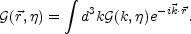
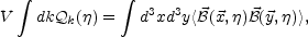
In order to understand correctly the argument under discussion the volume average of the magnetic energy density has to be introduced (see [150] for a lucid discussion on the various possible averages of large-scale magnetic fields and see [151] for a complementary point of view). A generic rotationally and parity invariant two-point function for the magnetic inhomogeneities can be written as

(5.96)

Defining now

(5.97)

From Eqs. (5.96)-(5.97) the following relation can be obtained

(5.98)

where _k() is related to (k, ) and V is the averaging volume.

The idea is now to study the scaling properties of _k() under the similarity transformations given in Eq. (5.95). Following [147], it is possible to show that

(5.99)

with = - 1 - 2. In Eq. (5.99) _k() is related to the magnetic energy density and F(x) is a function of the single argument x = (k^(3+)/2 ). If, initially, the spectrum of the magnetic energy density is k, then at later time the evolution will be dictated by F(x). Since a⁴() _k() is approximately constant, because of flux conservation, then the comoving momentum will evolve, approximately, as

(5.100)

while the physical momentum will scale like

(5.101)

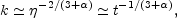
The conclusion of this argument is the following:

• if < -3 the cascade will be direct (or forward);

• if > -3 the comoving momentum moves toward the infra-red and the cascade will be inverse;

• if = -3, then, = 1 and, from Eqs. (5.95)-(5.99), the momentum and time dependence will be uncorrelated.

The Olesen scaling argument has interesting implications:

• if the initial spectrum of the magnetic energy density is concentrated at high momenta then, an inverse cascade is likely;

• from Eqs. (5.100) and (5.101) the typical correlation scale of the magnetic field may, in principle, evolve faster than in the case where the inverse cascade is not present.

In a FRW Universe the correlation scale evolves as () = (₀) a() from a given initial time ₀ where magnetic energy density is injected with spectral dependence k. If > -3, Eqs. (5.100)-(5.101) imply that

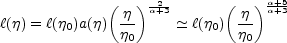(5.102)

where the second equality follows in a radiation dominated phase of expansion. In flat space, the analog of Eqs. (5.100)-(5.101) would imply that (t) ~ (t₀)(t / t₀)^2/(+3). Finally, in the parametrization of Olesen [147] the case of a Gaussian random field corresponds to = 2, i.e. = -3/2. In this case the correlation scale will evolve as

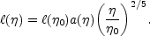(5.103)

In the context of hydrodynamics the scaling law expressed through Eq. (5.103) is also well known [153]. It is appropriate, at this point, to recall that Hogan [152] was the first one to discuss the evolution of the correlation scale produced by a Gaussian random injection spectrum (i.e. = 2). Hogan was also the first one to think of the first order phase transitions as a possible source of large scale magnetic fields [152].

An argument similar to the one discussed in the case of MHD can be discussed in the case of ordinary hydrodynamics. In this case, the analog of _k() will be related to the kinetic energy density whose spectrum, in the case of fully developed turbulence goes as k^-5/3, i.e. the usual Kolmogorov spectrum.

The evolution of the correlation scale derived in Eq. (5.103) can be obtained through another class of arguments usually employed in order to discuss inverse cascades in MHD: the mechanism of selective decay [87] which can be triggered in the context of magnetic and hydrodynamical turbulence. The basic idea is that modes with large wave-numbers decay faster than modes whose wavenumber is comparatively small. Son [142] applied these considerations to the evolution of large-scale magnetic fields at high temperatures and his results (when the magnetic field configuration has, initially, vanishing helicity) are in agreement with the ones obtained in [147, 148]. In [154] the topics discussed in [147, 142] have been revisited and in [155] the possible occurrence of inverse cascades has been criticized using renormalization group techniques.

The main assumption of the arguments presented so far is that the evolution of the plasma occurs in an inertial regime. As discussed above in this Section, at high temperatures the inertial regime is rather wide both from the magnetic end thermal points of view. However, in the case where the magnetic and thermal diffusivity scales are finite the arguments relying on the inertial regime cannot be, strictly speaking, applied. In this situation numerical simulations should be used in order to understand if the diffusive regime either precedes or follows the inverse cascade.

If the magnetic and thermal diffusivity scales are finite, two conceptually different possibilities can be envisaged. One possibility is that the inverse cascade terminates with a diffusive regime. The other possibility is that the onset of diffusion prevents the occurrence of the inverse cascade. This dilemma can be solved by numerical simulations along the lines of the ones already mentioned [145, 146]. The numerical simulations presented in [145, 146] are in (2 + 1) dimensions. The results support the occurrence of inverse cascade in the presence of large kinetic viscosity. The moment at which the cascade stops depends on the specific value of the viscosity coefficient. In [156, 157] (3 + 1)-dimensional MHD simulations have shown evidence of inverse cascade. Another possible limitation is that in the early Universe the magnetic and kinetic Reynolds numbers are both large and also their ratio, the Prandtl number, is very large. This feature seems to be difficult to include in simulations.

The considerations presented so far do not take into account the possibility that the initial magnetic field configuration has non vanishing helicity. If magnetic helicity is present the typical features of MHD turbulence can qualitatively change [87] and it was argued that the occurrence of inverse cascades may be even more likely [158, 159] (see also [160]). The conservation of the magnetic flux is now supplemented, in the magnetic sector of the evolution, by the conservation of the helicity obtained in Eqs. (4.25) and (4.27). The conservation of the helicity is extremely important in order to derive the MHD analog of Kolmogorov spectrum. In fact, the heuristic derivation of the Kolmogorov spectrum is based on the conservation of the kinetic energy density. If the conservation of the magnetic helicity is postulated, the same qualitative argument leading to the Kolmogorov spectrum will lead in the case of fully developed MHD turbulence to the so-called Iroshnikov-Kraichnan spectrum [87, 161, 162] whose specific form, is, in terms of the quantity introduced in Eq. (5.99) _k(₀) ~ k^-3/2.

Suppose, for simplicity, that the injection spectrum has a non-vanishing helicity and suppose that the helicity has the same sign everywhere. In this case ^. ~ ||². Since the helicity is conserved the magnetic field will scale according to Eqs. (5.95) but with = -1/2 corresponding to = 0. Hence, the correlation scale will evolve, in this case, as

(5.104)

i.e. faster than in the case of Eq. (5.103). It is difficult to draw general conclusions without specifying the nature and the features of the mechanism producing the injection configuration of the magnetic field. The results critically summarized in this Section will be important when discussing specific ideas on the origin of large-scale magnetic fields. In Fig. 5 the cases of different injection spectra are compared. It is clear that an injection spectrum given by a Gaussian random field leads to a rather inefficient inverse cascade. Since the magnetic helicity vanishes at the onset of the evolution, the rate of energy transfer from small to large scales is rather slow. On the contrary if the injection spectrum is helical, the rate increases significantly. For comparison the situation where the injection spectrum corresponds to the Iroshnikov-Kraichnan case, i.e. the case of fully developed MHD turbulence, is also reported. The dashed line of Fig. 5 illustrates the evolution of the correlation scale dictated by the the Universe expansion.

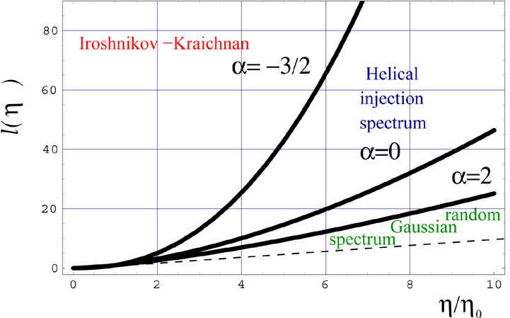Figure 5. The time evolution of the correlation scale is illustrated in the case of a FRW Universe dominated by radiation and in units 0 = 1. The case = 2 corresponds to the behaviour obtained in (5.103). The case = 2, corresponding to Eq. (5.104), refers to the situation of inverse cascade with an initial helical spectrum. For comparison the case = -3/2 is also reported. This last evolution takes place if the injection spectrum is of Iroshnikov-Kraichnan type.