1.4. STELLAR POPULATION ANALYSIS OF INDIVIDUAL GALAXIES

Having described the ways that stellar population models are being made, with some caveats about their capabilities, I will give some examples of their use in this sectionFrole, indicating a number of issues that one has to be aware of when applying them. I will first discuss stellar population analysis on colors, and then on line indices or continuous spectra.

1.4.1. The age-metallicity degeneracy and luminosity weighting

Determining both an age and a metallicity of a galaxy, or even of an SSP, is tougher than it seems. Galaxy colors become redder as the galaxy ages, since more stars move to the giant branch, and also for increasing metallicities, since the effective temperatures of most stars decrease because of increasing opacities in the stellar photosphere. Colors and many line strengths in the optical basically depend on the temperature of the main sequence turnoff. The effects of increasing the age can be compensated for many observables by decreasing the metallicity. Worthey (1994) estimated that a factor of 3 increase in metallicity corresponds to a factor of 2 in age when using optical colors as age indicators, the so-called 2/3 rule. Optical colours are notoriously degenerated (see Fig. 1.7 in the red part of the diagram).

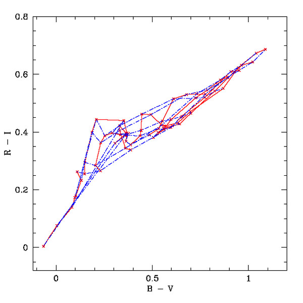Figure 1.7. The age-metallicity degeneracy as seen in a color-color diagram. Shown is a grid of SSPs with varying metallicity and age. Especially in the right part of the diagram age and metallicity cannot be determined independently for given observations of B-V and R-I. Used here are the MILES models (Vazdekis et al. 2010) with unimodal IMF and slope x = 1.3.

Both methods are being applied. For spectra covering only a small range in wavelength, very sophisticated indices have been developed maximizing age-sensitivity while minimizing the sensitivity to metallicity (e.g. Vazdekis & Arimoto 1999). In general, assuming that the stars in a galaxy are not coeval, a blue spectrum will give a different mean age than a red spectrum, since colors/indices in the blue will be more sensitive to the younger stars etc. This is the so-called luminosity weighting of stellar populations (I prefer not to use the term light weighting, since this has other associations, in e.g. material sciences). When applying stellar population synthesis codes, one should always realize that one's results have been weighted with the luminosity of the stars, implying that the brightest stars give the impression to be more important than they really are, when one weights according to mass, the natural choice. As an example, in the UV, sometimes 90% of the light in a cluster is coming from one star (Landsman et al. 1998) (see Fig. 1.8). This means that the mass-weighted age of that cluster could in principle be very old, while the luminosity weighted value is close the value for that star, i.e. young. For the interpretation of galaxy ages this distinction between mass and luminosity weighting is particularly important.

Figure 1.8. UIT image at ~ 1500Å and in V of the open cluster M67 (Landsman et al. 1998). Note that one star completely dominates the light in the UV.

1.4.2. Analysis using colors, and the role of extinction

In Chapter 1.3 we have found out that stellar populations in globular clusters are SSPs, and that populations in galaxies can be considered as linear combinations of SSPs. Recently, however, we have learned that the first assumption does not always hold. For a while it has been known that Cen, which up to now was considered to be a globular cluster, shows a spread in metallicity and possibly also age (Norris & Da Costa 1995). Conservative people could maintain for another 10 years that globular clusters have a single metallicity, by claiming that Cen is a galaxy, until recently Piotto et al. (2007), see Fig. 1.9, discovered multiple main sequences in the globular cluster NGC 2808. At the same time Mackey & Broby Nielsen found multiple main sequences in the LMC cluster NGC 1846. More clusters have been found later showing similar effects (e.g. Milone et al. 2008, Mackey et al. 2008). It is not clear yet what the reason is of these multiple branches. It could be that the He (or CNO) abundance is different, but also there might be a difference in age/metallicity. Spectroscopic studies here will have to show what really is happening.

Figure 1.9. Differential reddening corrected CMD of the globular cluster NGC 2808. In the inset some fits have been done with models of age 12.5 Gyr and various He abundances (from Piotto et al. 2007).

Color-magnitude diagrams can not only be used for globular clusters but also for galaxies in the rest of the Local Group. With HST it is possible to resolve individual stars below the Main Sequence Turnoff, and this way obtain exquisite star formation histories. In Fig. 1.10 I have reproduced a figure from the review of Tolstoy et al. (2009) with star formation histories of 3 dwarfs. An earlier, also excellent review, is by Mateo (1998). The star formation histories show that there are large variations between the galaxies of the local group, even between galaxies that have the same morphological classification (M32, NGC 205 and NGC 185). There are no galaxies for which we can exclude the presence of an underlying old population. Radial gradients in the populations of individual galaxies are seen as well. As mentioned before, more information about the abundance ratios in individual stars, giving information about star formation timescales, can be obtained from spectroscopy of bright giants in these galaxies.

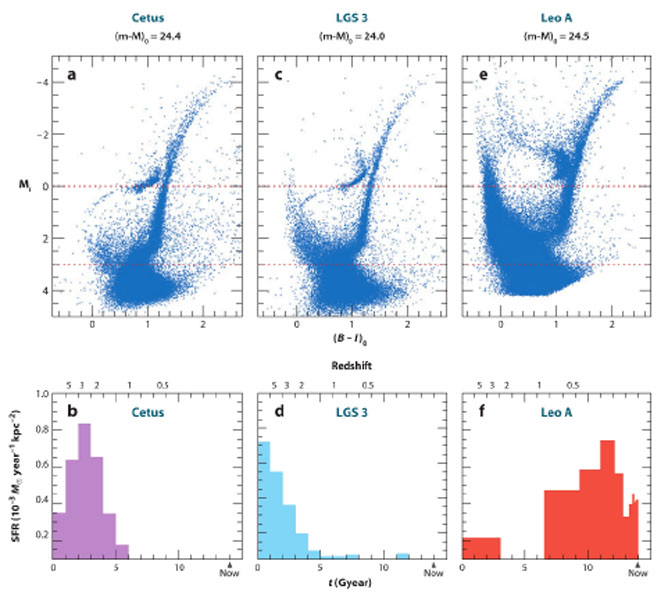Figure 1.10. HST/ACS color-magnitude diagrams SFHs for three Local Group dwarf galaxies: Cetus, a distant dwarf spheroidal galaxy, LGS 3, a transition-type dwarf galaxy and Leo A, a dwarf irregular. These results come from the LCID project (Gallart & the LCID team 2007, Cole et al. 2007). From Tolstoy et al. (2009).

When one goes further away, one can only resolve stars on the Red Giant Branch and beyond. One can obtain the spread in metallicity, e.g. in Centaurus A (Harris et al. 1999), and the galaxies in the ANGST survey (Dalcanton et al. 2009). A great application of counting the stars on the RGB is to use these star counts to make maps of the stellar density in the outer parts of galaxies. This way people have found huge low surface brightness features linking M31 with its companions, including M33, probably remains from encounters between these galaxies (Ibata et al. 2001, McConnachie et al. 2009). For the spiral galaxy NGC 300 Bland-Hawthorn et al. (2005) have been able to measure the stellar surface brightness profile to a distance of 10 effective radii from the galaxy center in this way.

In Fig. 1.11 a closeup is given of an RGB image of the disk of NGC 891, a nearby edge-on galaxy. What is clear are the many bright stars in the disk of the galaxy. Above it, many red filaments are seen. They are dust-lanes, seen up to large distances from the plane. In the lectures by Daniela Calzetti (this volume) you can see a lot of material about this dust, and how it extincts the light behind it. In Fig. 1.11 for example, further study shows that the blue stars seen in the left bottom corner are found in front of most of the disk of the galaxy, which itself is barely seen because of the extinction. In Fig. 1.12 one can see that the extinction is usually associated to spiral arms, and that it can be present to large radii. Here the extinction in a spiral disk is seen in front of an elliptical galaxy.

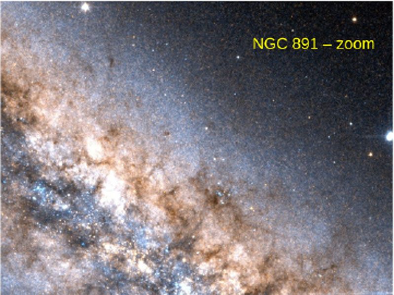Figure 1.11. Composite HST F814W/F555W image of NGC 891 (from the Hubble Legacy Archive). This galaxy is sometimes called the twin of our Milky Way. Note the young stars in the mid-plane and the dust extinction filaments.

Dust extinction is found predominantly in spiral galaxies of type Sab-Sc (e.g. Giovanelli et al. 1994). It is generally associated to molecular gas, and is stronger in larger (higher metallicity) galaxies. The UV energy absorbed by the dust is re-radiated in the IR and submm, responsible for a large fraction of the emission at those wavelengths. As far as stellar population synthesis is concerned the most important effect is that it reddens the colors using the dust extinction law (e.g. Cardelli et al. 1989). Reddening is strongest in the blue, and almost non-existent red-ward of 2 µm. In our Galaxy, it is impossible to see the Galactic Center in the optical, because of more than 20 magnitudes of extinction. However, in the infrared, at 2 micron, the extinction is only about 2 mag, so that observations there are easily possible. The ratio of reddening of dust in various colors is very similar to the effect of metallicity (and even age). This means that by simply measuring two colors, one cannot correct for the effects of extinction. For that more colors, or a spectrum are needed. It is therefore also not easy to measure the extinction from colors in a spiral galaxy. If one wants to do this, one can e.g. measure the amount of extinction statistically, by looking at the dependence on inclination. The color of a galaxy without extinction should not depend on inclination, while for an inclined galaxy the path length through the dust is longer, and thus the extinction. In Peletier et al. (1995) this technique is used to show that many nearby spiral galaxies in the B-band are optically thick within their central effective radius, but not in their outer parts. Certainly in bulges extinction plays a large role in many galaxies, and people analyzing the colors of external bulges should take this into account (e.g. Balcells & Peletier 1994).

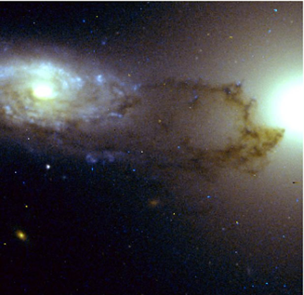Figure 1.12. Dust in a spiral galaxy seen in absorption in front of an elliptical galaxy (from White & Keel 1992).

In the absence of dust color-color diagrams consisting of an optical and an optical-IR (or IR) color, or, e.g., of a UV-Opt and an optical color, can be used to separate the effects of age and metallicity. This method is popular for globular clusters in nearby galaxies, for which high quality spectra are difficult to get. As can be seen in Fig. 1.13, it is important that accurate observational colors are available. Such studies can maybe explain the bi-modality in globular cluster colors (Ashman & Zepf 1992). Chies-Santos et al. (2012), for a sample of 14 early-type galaxies, found that, although the optical color distributions of the globular clusters are bimodal, this is not always the case in the infrared (z-K). The authors explain this results with a non-linear color-metallicity conversion, but clearly state that better data are required to confirm their results. This means that colors of globular clusters are not well understood. The, up to recently, firm conclusion that globular clusters have a bimodal metallicity distribution is now up for discussion.

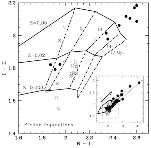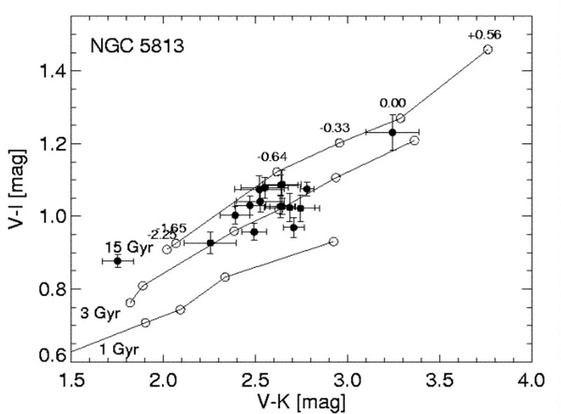
Figure 1.13. Top: V-I vs. V-K diagram for globular clusters in NGC 5813 (from Hempel et al. 2007). Bottom: B-I vs. I-H diagram for bulges of early-type spirals (from Peletier et al. 1999).

The same color combination is also often used for galaxy research. In Fig. 1.13 (right) HST data are shown of the inner parts of a sample of early-type spiral galaxies (Peletier et al. 1999), on top of a grid of SSP models. Central colors are indicated with red, filled symbols, while the colors at 0.5 bulge effective radii are indicated in open, blue circles. These latter colors are calculated on the minor axis of the bulge, on the side not obscured by the galaxy disk. Interesting to see from this plot is that most galaxy centers lie, often far, away from the model grid, indicating considerable amounts of extinction A_V of often more than 1 magnitude. The blue points cluster mostly together. Although the exact position of the model grid should be taken with caution (color differences are probably more reliable than exact colors, because of systematic effects in the models), this diagram seems to indicate that the bulges in this sample are old (mostly around 8-9 Gyr) with metallicities somewhat below solar.

The fact that one has to determine such detailed colors leads to another problem: the models. Up to recently, the spectrophotometric quality of the stellar population models has not been very high. In Sánchez-Blázquez et al. (2006) it is shown that the colors of stars in the MILES sample are consistent with their spectra within 1.5%, something which cannot be said from e.g. the Stelib library (Le Borgne et al. 2003), used for the Bruzual & Charlot (2003) models. Vazdekis and his group have extended the MILES library with a subset of good spectra from the Indo-US library (Valdes et al. 2004), with the aim of making a stellar library with wavelengths up to 9500Å with good flux calibration. In Ricciardelli et al. (2012) they show that, when fitting well-calibrated SDSS data, there are problems fitting the g-r vs. r-i distribution of galaxies for galaxies with high velocity dispersions. In this paper it is discussed that probably -enhanced stellar population models are needed to solve this issue.

1.4.3. Analysis using optical spectra

The main difference between a spectrum of a star and one of a composite system, such as a galaxy, is that the composite spectrum is the sum of many stellar spectra, weighted by their flux at the particular wavelength, and shifted by their individual radial velocities. These velocity shifts are not to be discarded. In a large galaxy stars move through one another with a velocity dispersion of about 300 km/s. This means that every line in the spectrum is broadened by a Gaussian with such a dispersion, which means that abundances can not be measured any more from narrow lines from single transitions, since those are all blended. Abundances have to be obtained by fitting stellar population models with given abundances to the galaxy spectra. Velocity broadening cannot be avoided, and we have to live with broadened lines. The most common way to measure line strengths in composite spectra is by using a system of line indices. These indices are defined by three pass-bands: a feature band, and two continuum bands, and measured as equivalent width: the surface (in Å ) under the spectrum that is normalized using the continuum on both sides (see Worthey et al. 1994 for definitions of the Lick/IDS system. In the Lick/IDS system 21 indices were defined to measure the strongest stellar features in the spectrum in the optical at a resolution of about 9Å (Worthey et al. 1994). 4 more indices (2 H and 2 H indices) were added in 1997 by Worthey & Ottaviani. These indices were used by Trager et al. (2000) to determine stellar population parameters from Lick/IDS indices of many nearby galaxies. Later-on, many more indices were added by Serven et al. (2005). Other indices are available in the literature. Rose (1994) defined several indices with a one-sided continuum, mainly in the blue. Cenarro et al. (2001) defined indices in the region of the Ca II IR triplet, sometimes with with multiple continuum regions. Normally an index becomes larger as the absorption line becomes stronger. Some lines, however, like the H and H lines in the Lick system, are situated in such crowded regions, that their continuum fluxes are affected by metal abundances, and that the line index sometimes can be negative, even though H or H is found in absorption.

Lick indices are hard to measure. Not only do they require the observed (galaxy) spectrum to be convolved to exactly the right resolution, and do they require a rather uncertain correction for velocity broadening, they also need certain zero point corrections to make sure that the instrumental response of the observed spectrum has the same shape as the Lick/IDS in the 1980's, when the standard stars for the Lick system were observed. This is a tedious job, since the Lick system does not work with flux calibrated spectra, and requires that for every observational setup a number of Lick standards are observed. To improve the situation, a slightly modified line index system (LIS) has been defined by Vazdekis et al. (2010). It is based on the MILES stellar library, uses the same wavelength definitions as the Lick/IDS system, and is defined on flux calibrated spectra, so that it is much easier for people to use this backward compatible system. To make it possible to also use less broad indices, for e.g. globular clusters and dwarf galaxies, the LIS system has been defined for standard resolutions of 5, 8.4 and 14 Å FWHM.

Although line indices are a good way to measure the strength of certain spectral features, there is, at present, no need any more to go through the indices, when comparing galaxy data with models, since one can directly fit the models to the data. Vazdekis (1999) already showed the power of this method, which dramatically can show regions of the spectrum where the models are inadequate (see Fig. 1.14). Of course, the stellar population models will have to be convolved with the correct LOSVD (Line of Sight Velocity Distribution), i.e. the broadening of the stars. The SAURON team (Sarzi et al. 2006) have applied full spectral fitting to Integral Field Spectroscopy of ellipticals and S0s, fitting the observed spectrum at every position in every galaxy with a set of SSP models, determining the LOSVD, and a best-fit stellar population model. They noticed that always large residuals occurred at the position of emission lines such as H and the [OIII] line at 5007Å. Realizing that they could at the same time also measure the velocity and broadening of the ionized gas, they then developed a method to fit at the same time velocity broadened SSP models and Gaussians representing the emission lines to the data. As a result, ionized gas could be found in 75% of the sample, much more than was previously known. This method is much more sensitive than e.g. methods that map emission lines using narrow-band filters. Of course, those latter methods can cover a larger area, at generally a higher spatial resolution.

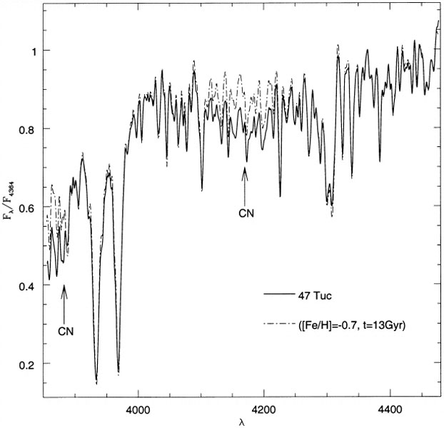Figure 1.14. Blue spectrum of 47 Tuc, together with an SSP fit by Vazdekis (1999). Marked are the well-known CN strong bands of this globular cluster.

Separating absorption and emission is in particular important for lines which are at the same time important absorption and emission lines, such as the Balmer lines H and H. These lines, which are so important to determine ages of stellar populations, can easily be filled in by emission. Before full spectral fitting was possible assumptions were made that the H emission line strength was a constant fraction of the [OIII] 5007Å line. The maps of Sarzi et al. (2006, 2010) show, however, that this ratio varies from galaxy to galaxy. Methods like this are so powerful that Balmer absorption line strengths can be measured in spiral galaxies with strong emission lines (e.g. Falcón-Barroso et al. 2006, MacArthur et al. 2009).

The most popular index-index diagram is the Mg b vs. H diagram. Here Mg b is mostly sensitive to metallicity, while H is mostly age-sensitive. Using this diagram it was found that massive galaxies have /Fe ratios higher than solar (Peletier 1989, Worthey et al. 1992). In Fig. 1.15 we show H against [MgFe50], a composite of the Lick indices Mg b and Fe 5015, from Kuntschner (2010). Here one sees how some relatively small differences between stellar population models can change the ages derived from these indices. Here the models of Schiavon (2007) and those of Thomas et al. (2003) are shown. The galaxies are from the SAURON sample of early-type galaxies, and are shown as lines, with a dot in the center. Using the models of Schiavon, the old galaxies (these are mostly the ellipticals and the massive S0's) are old everywhere, with metallicity decreasing outwards. If one uses the models of Thomas et al. (2003), the outer parts are older, with similar metallicity gradients. Note here that these ages are luminosity weighted ages, and that the younger galaxies probably consist of an older continuum with a young population superimposed.

Figure 1.15. Radial line strength gradients for the 48 early-type galaxies in the SAURON sample. The center of each galaxy is indicated by a filled circle and different colors are used for each galaxy. Over plotted are stellar population models by Schiavon (2007, left) and Thomas et al. (2003, right) for solar abundance ratios. Note that the latter models extend to [Z/H] = +0.67, whereas Schiavon models reach only [Z/H] = +0.2 (from Kuntschner et al. 2010).

Measuring element abundance ratios from integrated spectra is much less straightforward than for individual stars. What we know is that [Mg/Fe] varies strongly as a function of galaxy velocity dispersion (a proxy of mass). We also know that -elements vary more as a function of than Fe (Sánchez-Blázquez et al. 2006). From a sample of galaxies in the Coma cluster Smith et al. (2009) and Graves & Schiavon (2008) claim that the abundance ratios Mg/Fe and Ca/Fe simultaneously decrease with Fe/H and increase with . These dependences can be explained by varying star formation time scales as a function of , and therefore different ratios of element enrichment by SN type II and Ia. For both C/Fe and N/Fe, no correlation with Fe/H is observed at fixed . This can be explained if these elements are produced primarily by low/intermediate mass stars, and hence on a similar time-scale to the Fe enrichment. The element abundance ratio trends with [Fe/H] are very similar to those in our Galaxy, which suggests a high degree of regularity in the chemical enrichment history of galaxies (Smith et al. 2009).

1.4.4. Star Formation Histories and the SSP

The availability of full spectra makes it possible to recover the Star Formation History (SFH) in some detail. Here one can divide the efforts into 2 parts: efforts that fit the full spectrum, including UV and IR, using the far IR, originating mostly from dust emission, as well as the submm on one hand, and more detailed studies that determine the distribution of stars of various ages on the other. The most important result from the first kind of studies is the amount of hot, young stars, responsible for ionizing the gas end heating up the dust around them. For this work I refer to Daniela Calzetti's chapter in this book.

As far as the analysis of photospheric light is concerned, there is a growing body of full spectrum fitting algorithms that are being developed for constraining and recovering the Star Formation History (e.g., MOPED - Panter et al. 2003; Starlight - Cid Fernandes et al. 2005; Steckmap - Ocvirk et al. 2006; Koleva et al. 2008). SED fitting works best for large wavelength ranges. It is based on a set of SSP models and an extinction curve, and fits at the same time the stellar population mix, the LOSVD and the amount of extinction.

Using full spectrum fitting several independent bursts of star formation can be determined. The number of parameters that can be recovered from a spectrum depends strongly on the signal-to-noise ratio, wavelength coverage and presence or absence of a young population (Tojeiro et al. 2007). However, the results are strongly affected by the age-metallicity degeneracy, so interpreting the results is difficult. Also, there is a certain degeneracy between the number of components in the LOSVD, and the SFH. Some tests are shown in Ocvirk et al. (2008), who try to constrain at the same time the SFH and the LOSVD along the slit of the spiral galaxy NGC 4030. It is clear from this experiment that higher spectral resolution and S/N data is needed to obtain astrophysically reliable results which are not degenerate.

On the other hand, such studies are very useful to determine whether a galaxy is well fit by a one-SSP model, and if this is not the case, what the relative mass fraction in the various components in the SFH is. That information is useful to understand the formation history, combining it with spatial information about e.g. interactions. I will give 2 examples here.

The first is by Koleva et al. (2009). They derive star formation histories of dwarf ellipticals in the Fornax cluster using ESO-VLT data. To understand the formation of these galaxies, it is very important to know whether these star formation histories are extended or short-lived, and whether they are very diverse, as is the case in the Local Group. In the Fornax cluster the environment is different, with a stronger influence from the IGM. Usually the photometric images are featureless, so that little can be learned about the stellar populations from the morphological structure. The results show that the star formation histories are not very different from those in the Local Group, and vary from SSP-like to extended (Fig. 1.16).

Figure 1.16. Star formation histories for the inner arcsec of a number of dwarf ellipticals, from Koleva et al. (2009). Black lines indicate SFR obtained using Steckmap, green using ULYSS.

1.4.5. Learning about stellar populations using 2D spectroscopy

In the previous sections we have discussed how to derive the star formation history of a stellar population at a given position in a galaxy. One should always remember that galaxies are morphological and dynamical entities, and that the stellar populations that one derives are the result of the formation and evolution of the galaxy, and therefore intimately related to the morphological/kinematical component that one studies. 2-dimensional spectroscopy is an ideal tool to connect stellar populations with morphology and dynamics. In the last decade many of the large galaxies in the nearby Universe have been studied using the SAURON instrument at La Palma. The NIR Integral Field Spectrograph Sinfoni at ESO's VLT is making a large impact in the field at galaxy formation at z ~ 2 (SINS survey - Förster-Schreiber et al. 2009). Many IFU surveys are being planned (e.g. CALIFA, Sánchez et al. 2012; VIRUS, etc.).

The SAURON survey (de Zeeuw et al. 2002, Bacon et al. 2001) has shown that many early-type galaxies contain kinematically-defined central disks. H absorption maps often show that these disks contain stars that are younger than the stars in the main body of the galaxy. The connnection here between the stellar populations, the morphology and the kinematics shows us that these disks are formed later. Since most of the disks have angular momentum that has the same sign as that of the main galaxy, one thinks that the disks are formed from gas lost by stars in the galaxies themselves (Sarzi et al. 2006). Spiral galaxies, much more than elliptical galaxies, have several components, such as bulge, inner disk, outer disk, bars, rings, etc. Here studying the stellar populations together with morphology and dynamics much more enhances our understanding of all these components, and the galaxies as a whole. I will discuss here the inner regions of 2 spiral galaxies, in order of morphological type, from the SAURON study of Falcón-Barroso et al. (2006) and Peletier et al. (2007).

The first one is the Sa galaxy NGC 3623 (Fig. 1.17). The inner regions of this galaxy mainly contain old stellar populations, as shown by the absorption line maps and confirmed by the unsharp masked HST image, an image which is a very good indicator of dust extinction. Since young stars are always accompanied by extinction, unsharp masked images are an efficient way to find younger stars. However, the presence of dust is not always sufficient to detect young stars. The radial velocity map shows an edge-on, rotating disk in the center, confirmed by a central drop in the velocity dispersion. This central disk contains old stellar populations, probably slightly more metal rich (see the age and metallicity maps).

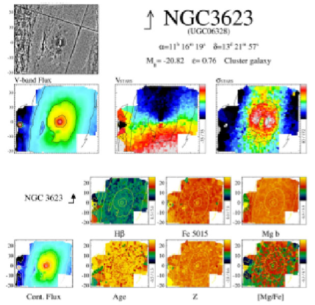Figure 1.17. 2-dimensional maps of various quantities in the inner regions of NGC 3623: (from top left to bottom right): unsharp masked HST image, V-band continuum image, stellar velocity field and velocity dispersion maps, H, Fe 5015 and Mg b absorption line maps, again V-band continuum image. age, metallicity and [Mg/Fe] map. All from SAURON (Falcón-Barroso et al. 2006, Peletier et al. 2007), except for the HST image.

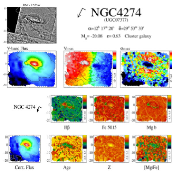
The next galaxy is also an Sab galaxy, NGC 4274 (Fig. 1.18). This galaxy seems not to be very different from the one before. The unsharp masked image shows a central spiral, which might be similar to the one in NGC 3623 (which is edge-on, so the spiral structure in the dust cannot be seen). This spiral is associated to a rotating feature, seen both in the velocity and the velocity dispersion maps. In both galaxies, ionized gas is present everywhere in the central regions (Falcón-Barroso et al. 2006). Different from NGC 3623, the stellar populations in the central disk in NGC 4274 are much younger than in the main body of the galaxy, as can be seen from the line strength maps, especially H absorption. If one now looks at the photometric decomposition (Peletier 2009), one sees that the part of the surface brightness profile of NGC 4274 that lies above the large exponential disk, i.e. the bulge, corresponds to the region of the inner disk, and is best fitted by a Sérsic profile with n = 1.3. In the case of NGC 3623 the so-defined bulge is much larger, and has a Sérsic index of n = 3.4. Kormendy & Kennicutt (2004) would call the bulge in NGC 4274 a pseudo-bulge, and the one in NGC 3623 a classical bulge. However, the comparison here shows that both objects are very similar, but that only the inner disk to elliptical bulge ratio in both galaxies is different. The study of other bulges in this sample shows that many early-type spiral galaxies contain central disks, with often young stellar populations in them.

Figure 1.18. Same as Fig. 1.17, but now for NGC 4274.

The study of the central stellar populations and dust can also be done very well using IRAC on the Spitzer Space Telescope. van der Wolk (2011) in his PhD Thesis presents color maps of these SAURON-selected spirals. Information about the ages of the stellar populations comes from the [3.6] - [4.5] maps (see Section 1.5.2). In Fig. 1.19 the [3.6] - [8.0] maps of the 2 galaxies are shown. These maps show the amount of warm dust (mainly due to PAHs). One can see that in NGC 3623 relatively little warm dust is present, consistent with the absorption line maps, while much more is present in NGC 4274.

Figure 1.19. Spitzer IRAC [3.6] - [8.0] color maps of the spiral galaxies NGC 3623 and NGC 4273 (from van der Wolk 2011). Shown are color maps of the whole galaxy, and a central zoom. This color, a good indicator of warm dust, shows a considerable amount of dust in the center of NGC 4274, corresponding to the region of the inner spiral in Fig. 1.18 and much less dust in the center of NGC 3623 (Fig. 1.17).

1.4.6. Stellar masses and the IMF in galaxies

Spectra and colors of SSPs are fairly insensitive to the initial mass function (IMF), because most of the light comes from stars in a narrow mass interval around the mass of stars at the main sequence turnoff. On one hand this is good, because it allows modelers to produce predictions for the spectra of galaxies that are accurate at most wavelengths. However, the same effect makes it possible to hide a large amount of mass in the form of low mass stars in a stellar population, making the stellar mass-to-light ratio a badly constrained parameter. Colors and lines of galaxies can generally be fitted well with a Salpeter IMF (a power law function with x = 1.3, see above). However, the same observables can also be fitted with an IMF that flattens below a certain critical mass, e.g. the Chabrier (2003) IMF, which flattens off below 0.6 M, giving a M/L ratio which is a factor 2 lower.

Until the end of the 1990's the uncertainties in the IMF were considered so important that estimates of stellar mass were rarely given. This changed with the influential paper by Bell & de Jong (2001), who showed that if one maximized the stellar mass in the disk when reproducing rotation curves of galaxies (the so-called maximum disk hypothesis) an IMF similar to the Salpeter IMF at the high-mass end with fewer low-mass stars, giving stellar M/L ratios 30% lower than the Salpeter value, was preferred. After this, it has become very common that stellar masses are given when fitting lines or colors of galaxies. In the important paper of Kauffmann et al. (2003), where stellar masses of many galaxies in the SDSS survey are calculated, the Kroupa (2001) IMF is used, a similar kind of IMF, and in only 2 sentences the authors mention that there can be systematic uncertainties in the derived stellar masses, as a result of the choice of the IMF.

Although in the optical most features are only slightly sensitive to the IMF-slope, there are some, mainly in the infrared, which strongly depend on the dwarf to giant ratio, i.e. the IMF-slope. Examples are the Wing-Ford band at 0.99 µm, the Na I doublet at 8190 Å, and the Ca II IR triplet around 8600Å. These lines have been used by several authors to constrain the IMF-slope (e.g., Spinrad & Taylor 1971, Faber & French 1980, Carter et al. 1986, Schiavon et al. 2000, Cenarro et al. 2003), but the results have never been very conclusive. The most important reason for this is that telluric absorption lines make it hard to measure accurate line strengths in this region of the spectrum. The second reason is that it is not always straightforward to derive the IMF-slope from the observations. For example, in Fig. 1.20 Cenarro et al. showed, based on the strength of the Ca II IR triplet and a molecular TiO index, and on the anti-correlation between the strength of the Ca II IR triplet and the velocity dispersion, that the IMF slope in elliptical galaxies increases for larger galaxies. However, other solutions are possible, e.g., that the [Ca/Fe] abundance ratio becomes lower for more massive galaxies. One might also think about systematic errors in the stellar population models that are needed to establish the IMF-slope. For example, in the models that Cenarro et al. use, solar abundance ratios are used in the stellar evolutionary calculations, and the stellar library used mostly consists of stars in the solar neighborhood, which implies that here too the abundance ratios must be close to solar.

Figure 1.20. SSPs model predictions at fixed old age with varying power-like IMF slopes (x = 0.3 -3.3, see the labels) and metallicity from -0.68 to 0.20. Different symbols indicate galaxies with different velocity dispersions (see Cenarro et al. 2003).

Recently, van Dokkum & Conroy (2010, 2011), and Conroy & van Dokkum (2012) have revived this topic. Using new methods to better remove the atmospheric absorption lines and new models in the near-infrared, they present conclusions that the IMF-slope increases with increasing galaxy velocity dispersion (mass). For the largest galaxies the IMFs found are a bit steeper than Salpeter (x = 1.6). This implies that stellar masses inferred from stellar population analysis will have to be increased by a small factor, which will not be larger than 2. Although this is an important result, one should remember the caveat that such a result depends on the stellar population models, which for non-solar abundance ratios are not perfect yet. Similar remarks can be made about the recent paper of Ferreras et al. (2012), who confirm Conroy & van Dokkum's result using the Na doublet at 8200Å with stacked data of a large sample of SDSS galaxies, and of Smith et al. (2012) who use an area near the Wing-Ford band. Recently, Cappellari et al. (2012) claim that independent analysis based on stellar dynamical fits to 2-D kinematic fits to galaxies of the Atlas-3d survey confirms the IMF trends observed in stellar populations.

If, when calculating stellar masses, one still doesn't want to depend on these estimates of the IMF slope, one can also use photometry or indices further to the infrared. For example, it is known that M/L ratios in the K-band vary little with stellar populations, since here the relative contribution to the light of dwarfs vs. giants is much smaller than in the optical. The same holds for the Spitzer [3.6] and [4.5] bands, which are still dominated by light from stars. Meidt et al. (2012) nicely show how stellar masses can be obtained from images in both these bands for spiral galaxies.

1.4.7. Beyond the optical

Stellar population synthesis in the UV is less well developed, because of various reasons. First of all, the amount of data available is limited, since it all has to come from space. Secondly, interpretation is complicated, since a few hot stars can over-shine all other stars, making it very difficult to obtain information on the not so young stellar populations.

Burstein et al. (1988) published a large number of IUE-spectra of early-type galaxies. Their main result was a relation between the 1550 - V color (1550 is here a passband with effective wavelength 1550Å ) and the optical Mg₂ index. Massive galaxies with large Mg₂ index have a very blue 1550 - V color. This effect, the so-called UV-upturn, is probably due to extreme horizontal branch stars, but can also have other reasons (see O'Connell 1999 and Yi 2008 for reviews). With new and better quality GALEX-data, Bureau et al. (2011) show that this effect is present only when the optical H index is low, which implies that from the optical spectrum there is no evidence for any young stellar populations (see Fig. 1.21.

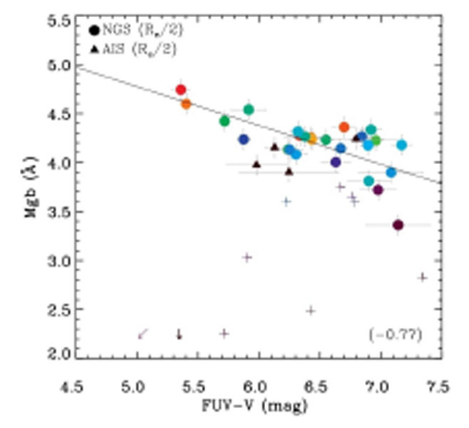Figure 1.21. Updated FUV - V vs. Mg b diagram (also called Burstein diagram), from Bureau et al. (2011). Galaxies with H > 1.8 Å are indicated with 'plus'-signs.

Very little has been done on the analysis of line strength indices. This is surprising, since the UV is particularly important for the analysis of high redshift spectra. Recently, Maraston et al. (2009) published some stellar population models based on the IUE-stellar library of Fanelli et al. (1992). A problem with this empirical library is, that its range in metallicity is small. However, in this region empirical stars are probably more reliable than synthetic spectra, due to difficulties treating the effect of stellar winds that affect the photospheric lines of massive stars. There are still considerable differences between using the Fanelli library and a high-resolution version of the Kurucz library of stellar spectra (Rodríguez-Merino et al. 2005) in the Maraston models.

There are ongoing efforts to develop a stellar library from HST/STIS stars, providing higher S/N and higher resolution spectra than IUE covering a much larger parameter space (the NGSL library - Gregg et al. 2006). This library has not been incorporated into any stellar population models yet, although it has been characterized and stellar parameters have been homogenized in Koleva & Vazdekis (2012).

Just like the UV, the near-IR has also not been studied very much. While broadband colors are predicted by many stellar population models, very few spectrophotometric models are available. The problem has been mentioned before. The NIR is dominated by evolved stellar populations, i.e., RGB and especially AGB, of which the number and lifetimes are not well known, since they are so short-lived that good statistics cannot be obtained from globular and open cluster HR-diagrams. Furthermore, AGB stars lose large amounts of mass, making their lifetimes and also their spectra uncertain. On top of that, they are highly variable. Spectrophotometric models at a resolution of ~ 1100 are available from Mouhcine & Lançon (2002). They are based on about 100 observed stars from Lançon & Wood (2000) for static luminous red stars, stars from Lançon & Mouhcine (2002) for oxygen rich and carbon rich LPVs, and the theoretical library of Lejeune et al. (1997, based on Kurucz models) in all other cases. Conroy & van Dokkum (2012) recently made some models using the IRTF library (Rayner et al. 2009, Cushing et al. 2005). At low resolution (~ 50Å ), there are models from Maraston (2005) and Charlot & Bruzual (Version of 2007, unpublished), based on theoretical atmospheres, and only tested in the broad bands J, H and K. Maraston also presents some low resolution indices. The problem with the models at present is that only the broad band fluxes have been tested well using clusters and galaxies, but that detailed testing of line indices or narrow band fluxes is still lacking. For example, in a recent paper, Lyubenova et al. (2012) showed that globular clusters cannot be fitted by the models of Maraston (2005) models in the C₂ - D_CO diagram. C₂ indicates the line strength of a feature at 1.77 µm (Maraston 2005), while D_CO is an index measuring the strength of the CO band head at 2.29 µm (Mármol-Queralto et al. 2008). The problem here is a lack of Carbon stars in the models, stars of ~ 1 Gyr (Lançon et al. 1999). It indicates that making models of the TP-AGB phase is very difficult (see also Marigo 2008). The situation might be improving soon. Better data of nearby galaxies and clusters are becoming available (e.g. Lyubenova et al. 2012, Silva et al. 2008, Mármol-Queralto et al. 2009). And better stellar libraries are expected (e.g., the X-Shooter library (Chen et al. 2011)). By comparing data with models, we will learn where the models should be improved, up to the moment that the NIR will give useful constraints to galaxy evolution theories.

1.4.8. Stellar population analysis from surface brightness fluctuations

In Fig. 1.22 one sees the nearby dwarf elliptical NGC 205 in 2 bands. In the redder band, F814W, the giants can be distinguished much more easily from the underlying mass of fainter stars than in F555W. One can imagine that if this galaxy is placed at larger distances, one can see the individual giants up to larger distances in F814W. One can use the noise map, obtained after removing a smooth model of the galaxy, as a measure of the galaxy distance. Even more, since this noise map strongly depends on the number of bright giants and supergiants, one can use the noise characteristics, or the surface brightness fluctuations as a way to characterize the stellar populations in a galaxy.

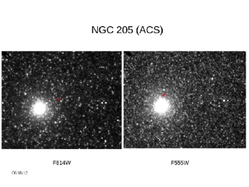Figure 1.22. The effect of surface brightness fluctuations: ACS images of NGC 205 in F814W (left) and F555W (right).

A review about surface brightness fluctuations as a stellar population indicator is given in Blakeslee (2009). It shows that the method can be used well for determining distances in early-type galaxies (giants or dwarfs), but that the use for stellar population analysis is still limited to the optical. In the near-IR there are considerable discrepancies between surface brightness fluctuations predicted by models and the observations (Lee et al. 2009). With the advent of new, large telescopes, this work will undoubtedly become more important in the future.