


With stellar population synthesis one wants to determine as much information from the stellar populations of an unresolved galaxy from a single spectrum as possible. Having seen how complicated our Milky Way is, it is clear that one cannot retrieve all the information that one would like to have. The integrated light contains contributions from stars with a large range in metallicity, mass and age, and even for stars of a fixed metallicity the relative distribution of elements might be different from one star to another. Since all this together is too much to obtain from a single spectrum, one often assumes an Initial Mass Function (IMF), the number of stars per mass interval at the moment that the stars were born, and tries to derive the star formation history (SFH) and the metallicity distribution of the stars in a galaxy.
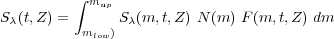
The spectrum of an integrated stellar population is obtained by integrating all stars along the line of sight.
 |
(1.1) |
Here S (m, t, Z) is the
spectral energy distribution (SED) of a star of mass m (going
from mup to mlow), age t and
metallicity Z, and F(m, t, z) the
flux in a normalizing band. The total galaxy spectrum is then obtained
by adding the contributions of the various ages and metallicities.
(m, t, Z) is the
spectral energy distribution (SED) of a star of mass m (going
from mup to mlow), age t and
metallicity Z, and F(m, t, z) the
flux in a normalizing band. The total galaxy spectrum is then obtained
by adding the contributions of the various ages and metallicities.
Modern stellar population synthesis assumes that the stellar populations in galaxies consist of a sum of Single Stellar Populations (SSP), building blocks of more complex stellar populations, entities that consist of all stars born at the same time, with the same metallicity. For example, galaxies do not consist only of A-stars of 2 solar mass, but stars of the full range of masses in the range of the IMF must exist. With this strong assumption, one can use stellar evolution theory to calculate the integrated properties of these SSPs, and then decompose the SED of galaxy into various SSPs. Justification of the SSP approach dates back from the time of Tinsley, who realized that clusters, both globular and open, could all be represented as single stellar populations. When looking at the nearest galaxies, the SSP approximation remains valid (Section 1.4.2). A nice overview of evolutionary stellar population models is given by Maraston (2005). Current SSP models predict full spectral energy distributions (SEDs) by integrating stellar spectra along theoretical isochrones. These spectra are selected from a stellar library, that consist of observations of real stars or of artificial spectra calculated using model atmospheres. Some of the presently most popular stellar population models are those by Worthey (1994), Maraston (2005), Bruzual & Charlot (2003) and later unpublished versions, Le Borgne et al. 2004 (Pégase HR), Leitherer et al. 2010 (Starburst99), Vazdekis et al. (2010), González Delgado et al. (2005) and Schiavon (2007).
Despite important progress in the last 2 decades, it is still not straightforward to routinely derive star formation histories and metallicity distributions from spectra. Here I will briefly indicate a number of reasons why this is the case, and in the coming sections I will elaborate on them. First of all, there is our relatively poor understanding of the advanced phases of stellar evolution, such as the supergiant phase and the asymptotic-giant-branch (AGB) phase. Stars in these phases are bright and short lived, so that they do contribute significantly to the spectrum of galaxies, but their numbers in color-magnitude diagrams of globular and open clusters are not large enough to constrain the fraction of light of these populations in the total spectrum. At the same time, mass loss, which is difficult to model, and is crucial for calculating their evolutionary path, plays such an important role in these stars, that it causes considerable uncertainties. Stars on the AGB contribute especially in the infrared, and in this region especially these uncertainties are most important.
A second, also very important problem is the age-metallicity degeneracy. In an integrated stellar population, the main effect of increasing the metallicity is raising the opacities of stars on the red giant branch (RGB), causing it to become redder, which implies that the integrated spectrum is redder, and that most strong atomic features in the optical are stronger, since they are stronger in cooler stars. The main effect of increasing the age is the same: the reddening of the RGB. This means that one can often not derive both age and metallicity at the same time: the so-called age-metallicity degeneracy. This degeneracy in fact can get worse: if there is dust in the galaxy, it will cause colors to become redder, acting in the same way as increasing metallicity or age. However, only colors are strongly affected by the effects of dust extinction. Line strengths are mostly not affected by extinction, except if blue and red continuum are lying very far away from each other. As a result, ages and metallicities are strongly degenerate, although there are ways to measure both parameters separately.
A third problem is that abundance ratios of galaxies are not always the
same as in the solar neighborhood. This shows up in our Galaxy as a
tight relation of [Mg/Fe] and metallicity [Fe/H]
(Edvardsson et
al. 1993).
It is thought that element formation is mainly taking place
in supernovae of type Ia and II. In explosions of SN type II (massive
stars) the amount of O and other
 -elements, as compared
to Fe,
that is produced is much larger than in SN of type Ia. It is believed
that during the formation of halo and bulge the number of SN type II
relative to type Ia was much higher than during the formation of the
disk, and as a result the ratio of Mg/Fe abundance is higher in our
Galactic halo and bulge than in the Galactic disk. Not only does the
fraction of -elements
relative to Fe vary. Variations are also
seen in the ratio of other elements to Fe (see the review of
Henry & Worthey
1999).
At present stellar population models (both the stellar
isochrones and the stellar libraries) rarely contain abundance
distribution other than solar. This means that several features in
observed galaxy spectra are not well fit by the best currently available
stellar population models.
-elements, as compared
to Fe,
that is produced is much larger than in SN of type Ia. It is believed
that during the formation of halo and bulge the number of SN type II
relative to type Ia was much higher than during the formation of the
disk, and as a result the ratio of Mg/Fe abundance is higher in our
Galactic halo and bulge than in the Galactic disk. Not only does the
fraction of -elements
relative to Fe vary. Variations are also
seen in the ratio of other elements to Fe (see the review of
Henry & Worthey
1999).
At present stellar population models (both the stellar
isochrones and the stellar libraries) rarely contain abundance
distribution other than solar. This means that several features in
observed galaxy spectra are not well fit by the best currently available
stellar population models.
1.3.1. Stellar evolution theory
The basic theory of stellar interiors is one of the eldest in astronomy. Already Eddington (1926) was able to somehow model the at that time just discovered Hertzsprung-Russel diagram with the differential equations for stellar interiors. Currently all models are in principle based on his theory, although they have been improved and expanded to take into account our growing understanding of the physics of stars. For details about the current stellar evolution models, see e.g. the book of Salaris & Cassisi (2006) on the Evolution of Stars and Stellar Populations. Many ideas in this book are reflected in the website of the BaSTI models (http://albione.oa-teramo.inaf.it/), by the previous authors and others. One might wonder why there is such a large variety of stellar models presented on this website. The reason is obvious: the input physics is so uncertain that the final fit to the data will have to show what choices should be made. The stellar evolution model traces the evolution of stars of given mass and chemical composition through the various evolutionary phases defined from the color-magnitude diagrams of open and globular clusters, and provides the basic stellar parameters - bolometric luminosities, effective temperatures and surface gravities as a function of the evolutionary time. Apart from the BaSTI models there are several other models available in the literature: e.g. the ones of Girardi et al. (2000), Marigo et al. (2008), Yi et al. (2003), Lejeune & Schaerer (2001), Dotter et al. (2007).
As far as the main stages of stellar evolution, it does not really
matter very much which models one takes (see an earlier comparison study
by
Charlot, Worthey &
Bressan 1996).
What matters are the
later evolutionary phases. For example, in the models of
Vandenberg et
al. (2000)
no overshooting is used. The models do not go
beyond the RGB, since the authors do not trust our understanding of the
physics beyond that phase. It has to do with the treatment of convection
and severe mass loss. The treatment of these phases (mainly the HB and
the TP-AGB) varies considerably between groups. The BaSTI models, for
example, give 2 sets of models for different mass loss rates
 . For
old stellar populations, for which the TP-AGB phase is unimportant, this
means that this uncertainty plays a smaller role (see
Mouhcine &
Lançon 2002.
In this paper it is shown that the fractional luminosity of
the AGB in J, H and K is the highest between
log(age) = 8.5 and 9.2, and reaches appr. 40% in J, 50% in
H and 60% in K. The contribution also goes up with
metallicity.). In the future larger telescopes will provide us
color-magnitude diagrams down to lower magnitudes, and the improved
statistics obtained in this way will probably cause the stellar
evolution calculations for these phases to considerably improve.
. For
old stellar populations, for which the TP-AGB phase is unimportant, this
means that this uncertainty plays a smaller role (see
Mouhcine &
Lançon 2002.
In this paper it is shown that the fractional luminosity of
the AGB in J, H and K is the highest between
log(age) = 8.5 and 9.2, and reaches appr. 40% in J, 50% in
H and 60% in K. The contribution also goes up with
metallicity.). In the future larger telescopes will provide us
color-magnitude diagrams down to lower magnitudes, and the improved
statistics obtained in this way will probably cause the stellar
evolution calculations for these phases to considerably improve.
Another source of uncertainty is the He contents of stars (indicated as mass fraction Y). He comes mainly from Big Bang Nucleosynthesis, but it strongly affected by H and He-burning in stars. An important problem is that there are no easy ways to determine the He-content in stars. Atomic transitions generally require high-energy photons, so are mostly found in hot stars, and are found in the blue or difficult to access UV. Since He does affect the location of the stellar evolution tracks (see e.g. the BaSTI models) this is an important problem. More generally, recent models assume that the helium fraction is related to the metallicity Z (e.g. Vazdekis et al. (2010) use Y = 0.23 + 2.25 Z).
Not only is there a problem with He, there are more than 100 other elements that each can have their own relative abundance w.r.t. Fe. Traditionally, these are parameterized with Z, the mass fraction of all elements other than H and He. Luckily, the relative abundances of these metals do not vary very much. This is because it is thought that element production is a fairly uniform process: it is done mostly in supernovae, but also in the envelopes of giant or supergiant stars. However, one knows that different types of supernovae produce different relative fractions of elements: for example, since the rate of element production depends on stellar mass, the relative distribution of elements ejected into the ISM in a SN explosion must also depend on mass. Element ratios affect the stellar population models in 2 ways: both the evolutionary tracks change position (see e.g. the BaSTI models), but more importantly, their line strengths change more directly (see e.g. Lee et al. 2009). In section 1.3.4 this item will be discussed in more detail.
A third problem is the IMF (see before), which is very difficult to measure. This point will be discussed in section 1.3.3 and section 1.4.6.
Other problems occur when converting theoretical parameters (Teff, g and abundances) to observational ones, such as colors or spectra. These problems are enormous. Although it seems straightforward to determine temperatures from spectra of observed stars, this is difficult for M-stars, which have such broad absorption lines that complicated procedures are required to determine them (e.g. Lançon et al. 2008). For most stars reasonably accurate gravities are available from distances and CM-diagram fitting, and they will become better when the results of GAIA are available. Determining abundances of stars is a complicated subject, which is mostly done comparing line strengths of isolated transitions with stellar atmosphere models (e.g. MARCS (Gustafsson et al. 2008)). See e.g. Ryde et al. 2004 for a review. In the ideal situation these isolated transitions are available. However, in practise for many elements no lines are available. Often, the resolution of the spectra is so low that one a few elements can be investigated, or that less accurate methods will have to be used, such as only determining a global metallicity for galaxies. For hot stars, such as O or B stars, determining abundances is particularly difficult, since they contain almost no lines.
Apart from the models described above, the BaSTI website also provides models for pre main sequence stars and for white dwarfs. The role of contact binary stars is not considered. One way for them of manifesting themselves is through Blue Straggler Stars (BSS), hydrogen-burning stars made hotter and more luminous by accretion and now residing in a region of the color-magnitude diagram normally occupied by much younger stars (e.g. Bond & MacConnell 1971). The fact that they have been found in globular clusters (Piotto et al. 2004) shows that their presence can be significant in galaxies. Recently, such blue stragglers have also been detected in the Galactic Bulge (Clarkson et al. 2011). The reason that historically not much attention has been given to BSS in stellar population models is that in color-magnitude (CM) diagrams Blue Straggler Stars are not found in large quantities, and that integrated models of old ages do fit elliptical galaxies. Since ignoring Blue Stragglers would cause elliptical galaxies to appear younger, it is worthwhile to study this issue in the future.
An important ingredient in stellar population models is the stellar library. The stellar library is essential for the models. Its spectral resolution and wavelength range determine the spectral resolution and wavelength range of the models. Its range in stellar types determines the applicability of the models, and to a large extent their quality. It is defined as a set of spectra of stars, covering a range in stellar parameters, i.e. effective temperature Teff, gravity g, and metallicity [Fe/H]. More recently, also abundance ratios, such as [Mg/Fe] are sometimes included (e.g. Milone et al. 2011). Stellar libraries can be theoretical (e.g. Hauschildt et al. (1997), Coelho et al. 2007) or empirical. Many of them can be found in the compilation of D. Montes (http://www.ucm.es/info/Astrof/invest/actividad/spectra.html). A good, but somewhat outdated review about empirical and theoretical stellar libraries is given by Coelho (2009). As mentioned in the section above, SSP model spectra are determined integrating the spectral contributions from stars along isochrones, and weighting them with the relative fraction of stars at every place along those isochrones. The required spectra here are obtained by selecting the star (or linear combination of a few stars) with the required temperature, gravity and metallicity. This is generally done using some kind of interpolation.
The first often used stellar library was the LICK-IDS library (Faber et al. 1985, Burstein et al. 1984, Gorgas et al. 1993, Worthey et al. 1994). This library consists of 425 spectra obtained with a non-linear Image Dissector Scanner, which each had been reduced to 25 low resolution line indices defined as equivalent widths of strong absorption lines in the spectrum. For large galaxies, for which the velocity dispersions are so large that many faint features in the spectrum are washed out, a considerable amount of information between 4200 and 6400 Å is contained in these indices. This library since then has been by far the most popular stellar library, and has been used many times to derive stellar population parameters of galaxies. Since the library is quite noisy, special fitting functions were made for every index, to facilitate the interpolation in the library when calculating SSP models (see e.g. Worthey et al. 1994).
With the advent of linear CCDs soon more accurate stellar libraries
became available, e.g. the library of
Jones et al. (1997),
which contains spectra, not just indices, covering 2 small wavelength
regions. This library was used by
Vazdekis (1999),
who created the first
stellar population models producing continuous output spectra. Now, 13
years later, among the most-used stellar libraries are MILES
(Sánchez-Blázquez
et al. 2006)
and Elodie
(Prugniel et al. 2007),
although many other libraries exist, especially in the
optical. The coverage of these libraries in terms of Teff and
log g is very good around solar metallicities. Outside the solar
metalliticy regime, the range of stellar population ages that can be
modeled is somewhat restricted. The main problem at the moment is, that
the wavelength range of these models is limited (e.g. the wavelength
coverage of MILES is 3500-7500Å), and that only Galactic stars are
included, most of them in the Galactic disk, implying that their
abundance ratios reflect the formation history of the Galactic disk,
with abundance ratios around solar. Recently, the MILES, CaT
(Cenarro et al. 2003)
and INDO-US libraries
(Valdes et al. 2004)
have been merged into the MIUSCAT library
(Vazdekis et al. 2012),
homogenizing resolution
and flux calibrating, extending the library to 9500Å. The
resolution of the current libraries goes from
R =  / = 40000 (Elodie) to
about 2.5Å(MILES). A higher resolution, but still unpublished
library is the UVES-POS stellar library (see
Bagnolo et al. 2003),
which has a resolution of 80000, but is not flux calibrated.
/ = 40000 (Elodie) to
about 2.5Å(MILES). A higher resolution, but still unpublished
library is the UVES-POS stellar library (see
Bagnolo et al. 2003),
which has a resolution of 80000, but is not flux calibrated.
In the near-UV and the NIR, spectral libraries are smaller, with smaller ranges in stellar parameter space, but the situation is rapidly improving. In the near-UV the best library is (and will remain for some time) NGSL, the Next Generation Spectral Library of Gregg, Silva and collaborators, containing spectra of 382 stars taken with HST/STIS at a wavelength-dependent resolution of 2000-10000, covering 1670-10250 Å with excellent flux calibration. In the NIR, a stellar library of 230 stars, the IRTF spectral library has recently become available: a compilation of stellar spectra that cover the wavelength range from 0.8 to 2.5 µm at a resolution of ~ 7Å and for some from 0.8 to 5.0 µm (Rayner et al. 2009; Cushing et al. 2005). The library, which has been flux calibrated using 2MASS photometry mainly consists of late-type stars (F-M), AGB, carbon and S stars, and L and T dwarfs. Most of the stars are of solar-metallicity. Apart from this there is the stellar spectra of cool giants (Lançon & Wood (2000), which contains ~ 100 stars taken at a resolution of R = 1100.
Theoretical stellar spectra are reasonably reliable for stars down to G-type, since in later types molecular bands, which are still hard to model, are starting to dominate the spectrum. Colors in the visible and near-IR bands are reproduced within the error bars for temperatures down to 3500K. At a resolution of R = 105 , the spectrum of the Sun is today reproduced to 5% of its relative flux, Arcturus (K1.5III) is reproduced to 9% and Vega (A0V) is reproduced to 1%. Residuals are in general larger towards cooler stars or lower surface gravities. For stars below 3500K, current developments in hydrodynamical models and pulsating atmospheres should improve the accuracy of the models, but it may well take some years before such grids are available to the completeness needed for population synthesis. For O- and B-type stars, recent developments in mass loss modeling, expanding atmospheres and wind features are being incorporated into the theoretical grids to model the UV with better accuracy (see Coelho 2009). Theoretical (or possibly semi-theoretical) libraries are the most promising to model the integrated spectral features of galaxies. As our understanding of stellar spectra improves, more and more analysis will be done with theoretical stellar libraries, especially in the optical and the near-UV. In the near-IR, I expect empirical libraries to remain highly superior for years to come. Progress should come from libraries with at the same time high spectral resolution and large wavelength coverage, such as the future X-Shooter spectral library XSL (Chen et al. 2011). By analyzing galaxies using at the same time optical, UV and near-IR features one should be able to constrain the old population dominating the mass, as well as recent or intermediate bursts of star formation at the same time.
1.3.3. The Initial Mass Function
An important ingredient in stellar population models is the Initial Mass Function. The IMF ultimately determines the mass to light ratio of a stellar population, and therefore choosing the right IMF is important to determine, among other things, the amount of dark matter in a galaxy.
Generally the IMF is determined by determining the mass function
of stars and correcting them for their evolution, to establish the
distribution of stars of a stellar population at birth. This can be done
for stars in the solar neighborhood, or in Galactic clusters. A huge
research effort has been invested to determine the shape and variability
of the IMF. Many details about this can be found in e.g. the review by
Kroupa (2007).
Salpeter (1955)
first described the IMF as a power-law, dN = c
m-
dm, where
dN is the number of stars in the mass interval m,
m + dm and c is the normalization constant. By
modelling the spatial distribution of the then observed stars with
assumptions on the star-formation rate, Galactic-disk structure and
stellar evolution time-scales, Salpeter determined
to be 2.35 for
0.4 < m < 10
M . Later
on, many other studies have extended the mass ranges to higher and lower
mass stars. The current situation is that the stellar IMF appears to be
extra-ordinarily universal, with an IMF which still has more or less
the same slope down to about 0.5
M, but turning over
towards lower masses (the Universal IMF of Kroupa, his equation (20),
see Fig. 1.4). Without such a turnover, the
amount of mass in a stellar population can become very large, which
often gets into conflict with dynamical measurements of mass in
galaxies, since those should be at least as large as the mass in stars
and stellar remnants. Kroupa also argues that the evidence for a
top-heavy IMF is not strong in well-resolved starburst clusters, and
that dynamical evolution of the clusters needs to be modelled in detail
to understand possibly deviant observed IMFs. For the low-mass end of
the IMF one has a reasonable idea of the IMF-slope down to about 0.2
M from star
counts in the solar neighborhood. Also,
here, the evidence for variations in the IMF is weak, although there
might be some speculative systematic variation with metallicity in the
sense that the more metal-poor and older populations may have flatter
MFs as expected from simple Jeans-mass arguments.
Bastian et al. (2010)
in a review for Annual Reviews in Astronomy and Astrophysics confirms
Kroupa's ideas: We do not find overwhelming evidence for large
systematic variations in the IMF as a function of the initial conditions
of star formation. We believe most reports of non-standard/varying IMFs
have other plausible explanations.
. Later
on, many other studies have extended the mass ranges to higher and lower
mass stars. The current situation is that the stellar IMF appears to be
extra-ordinarily universal, with an IMF which still has more or less
the same slope down to about 0.5
M, but turning over
towards lower masses (the Universal IMF of Kroupa, his equation (20),
see Fig. 1.4). Without such a turnover, the
amount of mass in a stellar population can become very large, which
often gets into conflict with dynamical measurements of mass in
galaxies, since those should be at least as large as the mass in stars
and stellar remnants. Kroupa also argues that the evidence for a
top-heavy IMF is not strong in well-resolved starburst clusters, and
that dynamical evolution of the clusters needs to be modelled in detail
to understand possibly deviant observed IMFs. For the low-mass end of
the IMF one has a reasonable idea of the IMF-slope down to about 0.2
M from star
counts in the solar neighborhood. Also,
here, the evidence for variations in the IMF is weak, although there
might be some speculative systematic variation with metallicity in the
sense that the more metal-poor and older populations may have flatter
MFs as expected from simple Jeans-mass arguments.
Bastian et al. (2010)
in a review for Annual Reviews in Astronomy and Astrophysics confirms
Kroupa's ideas: We do not find overwhelming evidence for large
systematic variations in the IMF as a function of the initial conditions
of star formation. We believe most reports of non-standard/varying IMFs
have other plausible explanations.
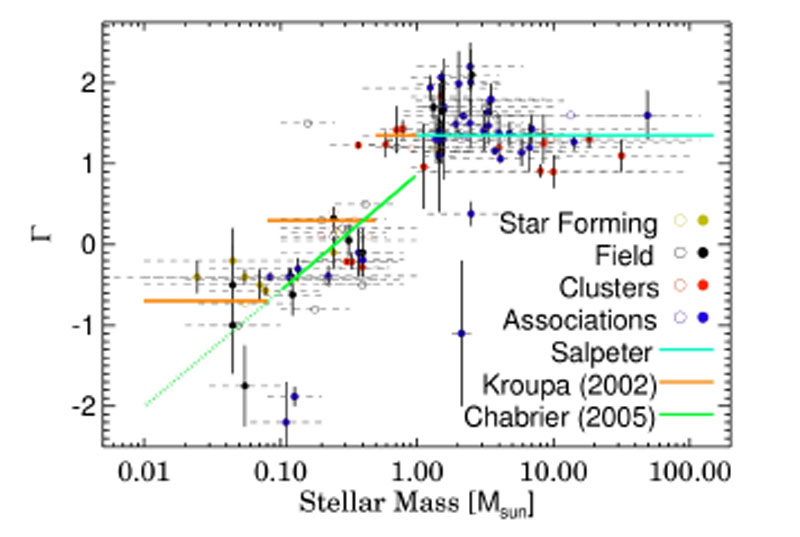 |
Figure 1.4. Derivative of the IMF-slope
( |
In Section 1.4.6 we will look at evidence for different types of IMFs based on integrated stellar populations. This evidence should be considered in the light of the above mentioned detailed work in our Galaxy.
Abundance ratios of elements in galaxies contain a wealth of information
about the way the stars were formed, and their formation
timescales. Element production for elements heavier than He is thought
to take place in stars. Explosions of supernovae and stellar mass loss
cause these newly formed atoms to enter the interstellar medium, where
they can be used to form new stars, which in turn can again enrich the
interstellar medium later. It is thought that Supernovae type II
(massive stars) and Ia (C-degenerate white dwarfs) are responsible for
most of the matter ejected into the ISM. SN type II eject mostly
so-called
-elements into the ISM
(see Fig. 1.5), i.e. O, Ne and Mg. SN type Ia,
which take longer to produce, since the stars first have to evolve to
their white dwarf phase, mainly produce Fe-peak elements. The fact that
the timescale of element production in these supernovae is so different
makes it possible to use the abundance ratio of an
-element and a Fe-peak
element as a star formation clock. A galaxy which forms all its
stars early-on will have a much higher
/Fe ratio than a galaxy
that forms its stars slowly.
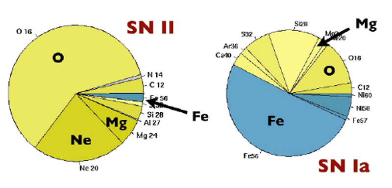 |
Figure 1.5. Supernova yields (= relative mass of metals released into the ISM at the death of the star), for SN type Ia and II. From Russell Smith, private communication. |
In our Galaxy it has been possible to measure abundances of many elements since almost 20 years (Edvardsson et al. 1993). This paper shows that the [Mg/Fe] ratio for disk stars is higher than solar for low metallicity stars, and at a certain metallicity starts to flatten off towards the solar value. This means that when our Galaxy was formed, and the metallicity of stars was low, they formed quickly. After a number of generations of metal enrichment, star formation became slower, and element production by SN type Ia started taking over. A nice review about abundances and abundance ratios in our Galaxy and in the Local Group is given by Tolstoy et al. (2009). In Fig. 1.6 the current status of Mg/Fe measurements in the Local Group is shown. Dwarf galaxies each have their own knee in the [Mg/Fe] vs. [Fe/H] diagram, indicating the start of SN Ia element formation. The position of the knee indicates the metal-enrichment achieved by a system at the time SN Ia start to contribute to the chemical evolution (e.g., Arimoto & Yoshii 1987, and modelled by e.g. Matteucci & Brocato, 1990). This is between 108 and 109 yr after the first star formation episode. A galaxy that efficiently produces and retains metals over this time frame will reach a higher metallicity by the time SN Ia start to contribute than a galaxy with a low star formation rate.
 |
Figure 1.6. Abundance ratios of Mg/Fe and Ca/Fe for the Milky Way and a few local group dwarfs (from Tolstoy et al. 2009). For the origin of the individual measurements see Tolstoy et al. 2009. |
Tolstoy et al. also explain that differences in relative abundances are
to be expected between various
-elements. Conditions
related to SN II explosions are responsible for the fact that O and Mg
often show different trends with [Fe/H] than Si, Ca and Ti (e.g.,
Fulbright, McWilliam
& Rich, 2007).
Apart from elements ejected into the ISM by SNe, also giant and
supergiant stars are responsible for the enrichment of the ISM.
For these evolved stars (giants or super-giants) material synthesized in
the core will have been mixed to the surface layers, and ejected into
the ISM through e.g. dust. Most of the material ejected in this way is
C, N and O.
The production of heavy neutron capture elements is less well understood. One distinguishes 2 processes, depending on the rate at which these captures occur, and are called the slow (s-) and the rapid (r-) process. The s-process occurs in low to intermediate-mass thermally pulsating AGB stars (see Travaglio et al., 2004, and references therein). R-process production is associated with massive star nucleosynthesis. More about these elements and possibilities about using their abundances as star formation clocks can be found in Tolstoy et al.
I will discuss abundance ratios from unresolved galaxies in Section 1.4.3.
 ) as a function of
stellar mass, derived from individual star counts (from
) as a function of
stellar mass, derived from individual star counts (from