2. THE ORIGIN OF STOCHASTICITY IN STELLAR POPULATION MODELLING

The stellar mass distribution in the fragmentation of a molecular cloud, even though it produces a discrete number of stars, has a continuous range of possible outcomes. Although we do not know the details of fragmentation and they vary from one cloud to another, we observe that the larger the stellar mass considered, the lower is the number of stars in the mass range near such a stellar mass. From the observed frequency distributions we make an abstraction to a continuous probability density distribution (statistical inference) such as the IMF or the stellar birth rate, which has proved to be a useful approach in characterizing this physical situation. By using such probability distributions, we construct the theory of stellar populations to obtain the possible luminosities of stellar ensembles (probabilistic description, the forward problem of predicting results) and produce a continuous family of probability distributions that vary according to certain parameters (mainly , t and Z). Finally, we compare these predictions with particular observations aimed at false regions of the parameter space; that is, to obtain combinations of , t and Z that are not compatible with observations (hypothesis testing in the space of observable luminosities).

The previous paragraph summarizes the three different steps in which stellar populations are involved. These three steps require stochastic (or random) variables, but, although related, each step needs different assumptions and distributions that should not be mixed up. Note that in the mathematical sense, a random variable is one that does not have a single fixed value, but a set of possible values, each with an associated probability distribution.

1. IMF inference. This is a statistical problem: inference of an unknown underlying probability distribution from observational data with a discrete number of events. This aspect is beyond the scope of our review. However, IMF inferences require correct visualization of the frequency distribution of stellar masses to avoid erroneous results (D'Agostino and Stephens 1986, Maíz Apellániz and Úbeda 2005). Such a problem in the visualization of distributions is general for inferences independently of the frequency distribution (stellar masses, distribution of globular clusters in a galaxy, or a set of integrated luminosities from Monte Carlo simulations of a system with given physical parameters).

2. Prediction of stellar population observables for given physical conditions. This is a probabilistic problem for which the underlying probability distribution, IMF and/or (m₀, t, Z) is obtained by hypothesis, since it defines the initial physical conditions. Such probability distributions are modified (evolved) to obtain a new set of probability distributions in the observational domain. The important point is that, in so far as we are interested in generic results, we must renounce particular details. We need a description that covers all possible stellar populations quantitatively, but not necessarily any particular one. This is reflected in the inputs used, which can only be modelled as probability distributions. Hence, we have two types of probability distributions: one defining the initial conditions and one defining observables.

   Regarding the initial conditions, the stellar mass is a continuous distribution and hence it cannot be described as a frequency distribution but as a continuous probability distribution, that is, a continuous probability density function (PDF). Hence, the IMF does not provide `the number of stars with a given initial mass', but, after integration, the probability that a star had an initial mass within a given mass range. If the input distribution refers to the probability that a star has a given initial mass, the output distribution must refer to the probability that a star has a given luminosity (at a given age and metallicity).

   For the luminosity of an ensemble of stars, we must consider all possible combinations of the possible luminosities of the individual stars in the ensemble. Again, this situation must be described by a PDF. In fact, the PDF of integrated luminosities is intrinsically related to the PDF that describes the luminosities of individual stars. A different question is how such a PDF of integrated luminosities is provided by synthesis models: these can produce a parametric description of the PDFs (traditional modelling), a set of luminosities from which the shape of the PDF can be recovered (Monte Carlo simulation), or an explicit computation of the PDF (self-convolution of the stellar PDF; see below).

3. Inference about the physical conditions from observed luminosities. This is a hypothesis-testing problem, which differs from statistical problems in the sense that it is not possible to define a universe of hypotheses. This implies that we are never sure that the best-fit solution is the actual solution. It is possible that a different set of hypotheses we had not identified might produce an even better fit. The only thing we can be sure of in hypothesis-testing problems is which solutions are incompatible with observed data. We can also evaluate the degree of compatibility of our hypothesis with the data, but with caution. In fact, the best ² obtained from comparison of models with observational data would be misleading; the formal solution of any ² fit is the whole ² distribution. Tarantola (2006) provide a general view of the problem, and Fouesneau et al. (2012) (especially Section 7.4 and Fig. 16) have described this approach for stellar clusters.

   Assuming the input distributions is correct and we aim to obtain only the evolutionary status of a system, we must still deal with the fact that the possible observables are distributed. An observed luminosity (or a spectrum) corresponds to a different evolutionary status and the distribution of possible luminosities (or spectra) is defined by the number of stars in our resolution element, . Since we have an accurate description of the distribution of possible luminosities as a PDF, the best situation corresponds to the case in which we can sample such a distribution of possible luminosities with a larger number of elements, n_sam, with the restriction that the total number of stars, N_tot, is fixed. As pointed out before, it is CMDs that have = 1 and n_sam = N_tot. We can understand now that the so-called sampling effects are related to n_sam and how we can take advantage of this by managing the trade-off between n_sam and . Note that the literature on sampling effects usually refers to situations in which N_tot has a low value; obviously, this implies that n_sam is low. However, that explanation loses the advantages that we can obtain by analysis of the scatter for the luminosities of stellar systems.

In summary, any time a probability distribution is needed, and such a probability distribution is reflected in observational properties, the description becomes probabilistic. Stochasticity, involving descriptions in terms of probability distributions, is intrinsic to nature and is implicit in the modelling of stellar populations. It can be traced back to the number of available stars sampled for the IMF or the (m₀, t, Z) distributions, but it is misleading to talk about IMF or stellar-birth-rate sampling effects, since these input distributions are only half of the story.

2.1. From the stellar birth rate to the stellar luminosity function

The aim of stellar population modelling is to obtain the evolution of observable properties for given initial conditions (m₀, t, Z). The observable property may be luminosities in different bands, spectral energy distributions, chemical yields, enrichment, or any parameter that can be related to stellar evolution theory. Thus, we need to transform the initial probability distribution (m₀, t, Z) in the PDF of the observable quantities, ℓ_i, at a given time, t_mod. In other words, we need to obtain the probability that in a stellar ensemble of age t_mod, a randomly chosen star has given values of ℓ₁, ..., ℓ_n. Let us call such a PDF (ℓ₁, ...,ℓ_n; t_mod), which is the theoretical stellar luminosity function. The stellar luminosity function is the distribution needed to describe the stellar population of a system.

Any stellar population models (from CMD to integrated luminosities or spectra), as well as their applications, have (ℓ₁, ...,ℓ_n;t_mod) as the underlying distribution. (m₀, t, Z) and stellar evolution theory are the gateway to obtaining (ℓ₁, ...,ℓ_n; t_mod). However, in most stellar population studies, (ℓ₁, ...,ℓ_n;t_mod) is not computed explicitly; it is not even taken into consideration, or even mentioned. Neglecting the stellar luminosity function as the underlying distribution in stellar population models produces tortuous, and sometimes erroneous, interpretations in model results and inferences from observational data.

There are several justifications for not using (ℓ₁, ...,ℓ_n; t_mod); it is difficult to compute explicitly (see below) and it is difficult to work in an n-dimensional space in both the mathematical and physical senses. We can work directly with (m₀, t, Z) and stellar evolution theory and isochrones, ℓ_i(m₀; , Z), where is the time measured since the birth of the star, without explicit computation of (ℓ₁, ...,ℓ_n;t_mod). In the following paragraphs I present a simplified description of a simple luminosity (ℓ t_mod). Such a description is enough for understanding most of the results and applications of stellar population models.

First, the physical conditions are defined by (m₀, t, Z) but we must obtain the possible luminosities at a given t_mod. When t_mod is greater than the lifetime of stars above a certain initial mass, the first component of (ℓ t_mod) is a Dirac delta function at ℓ = 0 that contains the probability that a randomly chosen star taken from (m₀, t, Z) is a dead star at t_mod. With regard to isochrones, dead stars are rarely in the tables in so far as only luminosities are included. However, they are included if the isochrone provides the cumulative ejection of chemical species from stars of different initial masses (as needed for chemical evolution models).

Second, stars in the MS are described smoothly by ℓ(m₀; , Z), which are monotonic continuous functions. In this region there is a one-to-one relation between ℓ and m₀, so (ℓ t_mod) resembles (m₀, t, Z). For an SSP case with a power law IMF, (ℓ t_mod) is another power law with a different exponent.

Third, discontinuities in ℓ(m₀; , Z) lead to discontinuities or bumps in (ℓ t_mod). Depending on luminosities before ℓ(m_0-; , Z) and after ℓ(m₀₊; , Z), they lead to a gap in the distribution (when ℓ(m_0-; , Z) < ℓ(m₀₊; , Z)), or an extra contribution to ℓ(m₀₊; , Z) (when ℓ(m_0-; , Z) > ℓ(m₀₊; , Z)). Discontinuities are related to changes in stellar evolutionary phases as a function of the initial mass, and to intrinsic discontinuities of stellar evolution (e.g. stars on the horizontal branch).

Fourth, variations in the derivative of ℓ(m₀; , Z) led to depressions and bumps in (ℓ t_mod). Consider a mass range for which a small variation in m₀ leads to a large variation in ℓ (the so-called fast evolutionary phases). We must cover a large ℓ range with a small range of m₀ values; hence, there will be a lower probability of finding stars in the given luminosity range (and in such an evolutionary phase), and hence a depression in (ℓ t_mod). The steeper the slope, the deeper is the depression. Conversely, when the slope of ℓ(m₀; , Z) is flat, there is a large mass range sharing the same luminosity; hence, it is easier to find stars with the corresponding ℓ values, and the probability for such ℓ values increases. Both situations are present in PMS phases.

In summary: (a) (ℓ₁, ...,ℓ_n; t_mod) has three different regimes, a Dirac delta component at zero luminosity because of dead stars, a low luminosity regime corresponding to the MS that resembles (m₀, t, Z), and a high luminosity regime primarily defined by the PMS evolution that may overlap the MS regime; and (b) the lower the possible evolutionary phases in the PMS, the simpler is (ℓ₁, ...,ℓ_n; t_mod). In addition, the greater the possible evolutionary phases, the greater is the possibility of the incidence of bumps and depressions in the high-luminosity tail of the distribution.

2.2. From resolved CMD to integrated luminosities and the dependence on

The previous section described the probability distribution that defines the probability that a randomly chosen star in a given system with defined (m₀, t, Z) at time t_mod has given values of luminosity ℓ₁, ...,ℓ_n. Let us assume that we now have a case in which we do not have all the stars resolved, but that we observe a stellar system for which stars have been grouped (randomly) in pairs. This would be a cluster in which single stars are superposed or blended. The probability of observing an integrated luminosity L_{i, = 2} from the sum for two stars is given by the probability that the first star has luminosity of ℓ_i multiplied by the probability that the second star has luminosity of L_{i, = 2} - ℓ_i considering all possible ℓ_i values; that is, convolution of the stellar luminosity function with itself (Cerviño and Luridiana 2006). Following the same argument, it is trivial to see that the PDF describing the integrated luminosity of a system with stars, (L₁, ...,L_n; t_mod), is the result of self-convolutions of (ℓ₁, ...,ℓ_n; t_mod).

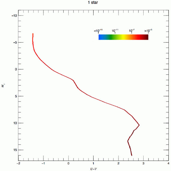
The situation in a U - V versus M_V Hess diagram is illustrated in Fig. 2 for = 1, 2, 64 and 2048. The figure is from Maíz Apellániz (2008), who studied possible bias in IMF inferences because of crowding and used the convolution process already described. The figure uses logarithmic quantities; hence, it shows the relative scatter, which decreases as increases. An important feature of the plot is that the case with a larger number of stars shows a banana-like structure caused by correlation between the U and V bands. In terms of individual stars, those that dominate the light in the V band are not exactly the same as those that dominate the light in the U band. However, there is partial correlation between the two types of stars resulting from (m₀, t, Z). Such partial correlation is present when stars are grouped to obtain integrated luminosities. These figures also illustrate how CMD studies ( = 1) can be naturally linked to studies of integrated luminosities ( > 2) as long as we have enough observations (n_sam) to sample the CMD diagram of integrated luminosities.

Figure 2. U - V L versus MV Hess diagram for a zero-age SSP system with = 1 (top left), = 2 (top right), = 64 (bottom left) and = 2048 (bottom right) based on work by Maíz Apellániz (2008). Figure courtesy of J. Maíz Apellániz.