5. REGULATION OF STAR FORMATION IN GMCs

Our discussion thus far provides the framework to address the final topic of this review: what are the dominant interstellar processes that regulate the rate of star formation at GMC and galactic scales? The accumulation of GMCs is the first step in star formation, and large scale, top-down processes appear to determine a cloud's starting mean density, mass to magnetic flux ratio, Mach number, and boundedness. But are these initial conditions retained for times longer than a cloud dynamical time, and do they affect the formation of stars within the cloud? If so, how stars form is ultimately determined by the large scale dynamics of the host galaxy. Alternatively, if the initial state of GMCs is quickly erased by internally-driven turbulence or external perturbations, then the regulatory agent of star formation lies instead on small scales within individual GMCs. In this section, we review the proposed schemes and key GMC properties that regulate the production of stars.

5.1. Regulation Mechanisms

Star formation occurs at a much lower pace than its theoretical possible free-fall maximum (see Section 2.6). Explaining why this is so is a key goal of star formation theories. These theories are intimately related to the assumptions made about the evolutionary path of GMCs. Two theoretical limits for cloud evolution are a state of global collapse with a duration ~ _ff and a quasi-steady state in which clouds are supported for times ≫ _ff.

In the global collapse limit, one achieves low SFRs by having a low net star formation efficiency _* over the lifetime ~ _ff of any given GMC, and then disrupting the GMC via feedback. The mechanisms invoked to accomplish this are the same as those invoked in Section 4.2.3 to drive internal turbulence: photoionization and supernovae. Some simulations suggest this these mechanisms can indeed enforce low _*: Vázquez-Semadeni et al. (2010) and Colín et al. (2013), using a subgrid model for ionizing feedback, find that _* 10% for clouds up to ~ 10⁵ M, and (Zamora-Avilés et al. 2012) find that the evolutionary timescales produced by this mechanism of cloud disruption are consistent with those inferred in the Large Magellanic Cloud (Section 2.5). On the other hand, it remains unclear what mechanisms might be able to disrupt ~ 10⁶ M clouds.

If clouds are supported against large-scale collapse, then star formation consists of a small fraction of the mass "percolating" through this support to collapse and form stars. Two major forms of support have been considered: magnetic (e.g., Shu et al. 1987, Mouschovias 1991a, b) and turbulent (e.g., Mac Low and Klessen 2004, Ballesteros-Paredes et al. 2007). While dominant for over two decades, the magnetic support theories, in which the percolation was allowed by ambipolar diffusion, are now less favored, (though see Mouschovias et al. 2009, Mouschovias and Tassis 2010) due to growing observational evidence that molecular clouds are magnetically supercritical (Section 2.4). We do not discuss these models further.

In the turbulent support scenario, supersonic turbulent motions behave as a source of pressure with respect to structures whose size scales are larger than the largest scales of the turbulent motions (the “energy containing scale” of the turbulence), while inducing local compressions at scales much smaller than that. A simple analytic argument suggests that, regardless of whether turbulence is internally- or externally-driven, its net effect is to increase the effective Jeans mass as M_J,turb ∝ v_rms², where v_rms is the rms turbulent velocity (Mac Low and Klessen 2004). Early numerical simulations of driven turbulence in isothermal clouds (Klessen et al. 2000, Vázquez-Semadeni et al. 2003) indeed show that, holding all other quantities fixed, raising the Mach number of the flow decreases the dimensionless star formation rate _ff. However, this is true only as long as the turbulence is maintained; if it is allowed to decay, then raising the Mach number actually raises _ff, because in this case the turbulence simply accelerates the formation of dense regions and then dissipates (Nakamura and Li 2005). Magnetic fields, even those not strong enough to render the gas subcritical, also decrease _ff (Heitsch et al. 2001, Vázquez-Semadeni et al. 2005, Padoan and Nordlund 2011, Federrath and Klessen 2012).

To calculate the SFR in this scenario, one can idealize the turbulence level, mean cloud density, and SFR as quasi-stationary, and then attempt to compute _ff. In recent years, a number of analytic models have been developed to do so (Krumholz and McKee 2005, Padoan and Nordlund 2011, Hennebelle and Chabrier 2011; see Federrath and Klessen 2012 for a useful compilation, and for generalizations of several of the models). These models generally exploit the fact that supersonic isothermal turbulence produces a probability density distribution (PDF) with a lognormal form (Vazquez-Semadeni 1994), so that there is always a fraction of the mass at high densities. The models then assume that the mass at high densities (above some threshold), M_hd, is responsible for the instantaneous SFR, which is given as SFR = M_hd / , where is some characteristic timescale of the collapse at those high densities.

In all of these models _ff is determined by other dimensionelss numbers: the rms turbulent Mach number , the virial ratio _G, and (when magnetic fields are considered) the magnetic parameter; the ratio of compressive to solenoidal modes in the turbulence is a fourth possible parameter (Federrath et al. 2008, Federrath and Klessen 2012). The models differ in their choices of density threshold and timescale (see the chapter by Padoan et al.), leading to variations in the predicted dependence of _ff on , _G, and . However, all the models produce _ff ~ 0.01 - 0.1 for dimensionless values comparable to those observed. Federrath and Klessen (2012) and Padoan et al. (2012) have conducted large campaigns of numerical simulations where they have systematically varied , _G, and , measured _ff, and compared to the analytic models. Padoan et al. (2012) give their results in terms of the ratio t_ff / t_dyn rather than _G, but the two are identical up to a constant factor (Tan et al. 2006). In general they find that _ff decreases strongly with _G and increases weakly with , and that a dynamically-significant magnetic field (but not one so strong as to render the gas subcritical) reduces _ff by a factor of ~ 3. Simulations produce _ff ~ 0.01 - 0.1, in general agreement with the range of analytic predictions.

One can also generalize the quasi-stationary turbulent support models by embedding them in time-dependent models for the evolution of a cloud as a whole. In this approach one computes the instantaneous SFR from a cloud's current state (using one of the turbulent support models or based on some other calibration from simulations), but the total mass, mean density, and other quantities evolve in time, so that the instantaneous SFR does too. In this type of model, a variety of assumptions are necessarily made about the cloud's geometry and about the effect of the stellar feedback. Krumholz et al. (2006) and Goldbaum et al. (2011) adopt a spherical geometry and compute the evolution from the virial theorem, assuming that feedback can drive turbulence that inhibits collapse. As illustrated in Figure 7, they find that most clouds undergo oscillations around equilibrium before being destroyed at final SFEs ~ 5-10%. The models match a wide range of observations, including the distributions of column density, linewidth-size relation, and cloud lifetime. In constrast, Zamora-Avilés et al. (2012, also shown in Figure 7) adopt a planar geometry (which implies longer free-fall times than in the spherical case; Toalá et al. 2012) and assume that feedback does not drive turbulence or inhibit contraction. With these models they reproduce the star formation rates seen in low- and high-mass clouds and clumps, and the stellar age distributions in nearby clusters. As shown in the Figure, the overall evolution is quite different in the two models, with the Goldbaum et al. clouds undergoing multiple oscillations at roughly fixed and M_* / M_gas, while the Zamora-Avilés et al. model predicts a much more monotonic evolution. Differentiating between these two pictures will require a better understanding of the extent to which feedback is able to inhibit collapse.

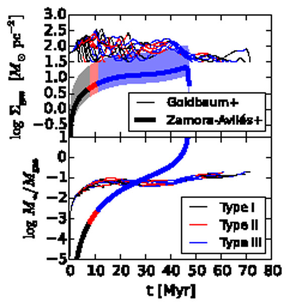Figure 7. Predictions for the large-scale evolution of GMCs using the models of Goldbaum et al. (2011, thin lines, each line corresponding to a different realization of a stochastic model) and Zamora-Avilés et al. (2012, thick line). The top panel shows the gas surface density. The minimum in the Goldbaum et al. models is the threshold at which CO dissociates. For the planar Zamora-Avilés et al. model, the thick line is the median and the shaded region is the 10th - 90th percentile range for random orientation. The bottom panel shows the ratio of instantaneous stellar to gas mass. Colors indicate the type following the Kawamura et al. (2009) classification (see Section 2.5), computed based on the H and V-band luminosities of the stellar populations.

5.2. Connection Between Local and Global Scales

Extraglactic star formation observations at large scales average over regions several times the disk scale height in width, and over many GMCs. As discussed in Section 2.1, there is an approximately linear correlation between the surface densities of SFR and molecular gas in regions where _gas 100 M pc^-2, likely because observations are simply counting the number of GMCs in a beam. At higher _gas, the volume filling factor of molecular material approaches unity, and the index N of the correlation _SFR ∝ _gas^N increases. This can be due to increasing density of molecular gas leading to shorter gravitational collapse and star formation timescales, or because higher total gas surface density leads to stronger gravitational instability and thus faster star formation. At the low values of _gas found in the outer disks of spirals (and in dwarfs), the index N is also greater than unity. This does not necessarily imply that there is a cut-off of _SFR at low gas surface densities, although simple models of gravitational instability in isothermal disks can indeed reproduce this result (Li et al. 2005), but instead may indicate that additional parameters beyond just _gas control _SFR. In outer disks, the ISM is mostly diffuse atomic gas and the radial scale length of _gas is quite large (comparable to the size of the optical disk; Bigiel and Blitz 2012). The slow fall-off of _gas with radial distance implies that the sensitivity of _SFR to other parameters will become more evident in these regions. For example, a higher surface density in the old stellar disk appears to raise _SFR (Blitz and Rosolowsky 2004, 2006, Leroy et al. 2008), likely because stellar gravity confines the gas disk, raising the density and lowering the dynamical time. Conversely, _SFR is lower in lower-metallicity galaxies (Bolatto et al. 2011), likely because lower dust shielding against UV radiation inhibits the formation of a cold, star-forming phase (Krumholz et al. 2009b).

Feedback must certainly be part of this story. Recent large scale simulations of disk galaxies have consistently pointed to the need for feedback to prevent runaway collapse and limit star formation rates to observed levels (e.g., Kim et al. 2011, Tasker 2011, Hopkins et al. 2011, 2012, Dobbs et al. 2011a, Shetty and Ostriker 2012, Agertz et al. 2013). With feedback parameterizations that yield realistic SFRs, other ISM properties (including turbulence levels and gas fractions in different H i phases) are also realistic (see above and also Joung et al. 2009, Hill et al. 2012). However, it still also an open question whether feedback is the entire story for the large scale SFR. In some simulations (e.g., Ostriker and Shetty 2011, Dobbs et al. 2011a, Hopkins et al. 2011, 2012, Shetty and Ostriker 2012, Agertz et al. 2013), the SFR on 100 pc scales is mainly set by the time required for gas to become gravitationally-unstable on large scales and by the parameters that control stellar feedback, and is insensitive to the parameterization of star formation on pc scales. In other models the SFR is sensitive to the parameters describing both feedback and small-scale star formation (e.g., _ff and H₂ chemistry; Gnedin and Kravtsov 2010, Gnedin and Kravtsov 2011, Kuhlen et al. 2012, Kuhlen et al. 2013).

Part of this disagreement is doubtless due to the fact that current simulations do not have sufficient resolution to include the details of feedback, and in many cases they do not even include the required physical mechanisms (for example radiative transfer and ionization chemistry). Instead, they rely on subgrid models for momentum and energy injection by supernovae, radiation, and winds, and the results depend on the details of how these mechanisms are implemented. Resolving the question of whether feedback alone is sufficient to explain the large-scale star formation rate of galaxies will require both refinement of the subgrid feedback models using high resolution simulations, and comparison to observations in a range of environments. In at least some cases, the small-scale simulations have raised significant doubts about popular subgrid models (e.g., Krumholz and Thompson 2012, Krumholz and Thompson 2013).

A number of authors have also developed analytic models for large-scale star formation rates in galactic disks. Krumholz et al. (2009b) propose a model in which the fraction of the ISM in a star-forming molecular phase is determined by the balance between photodissociation and H₂ formation, and the star formation rate within GMCs is determined by the turbulence-regulated star formation model of Krumholz and McKee (2005). This model depends on assumed relations between cloud complexes and the properties of the interstellar medium on large scales, including the assumption that the surface density of cloud complexes is proportional to that of the ISM on kpc scales, and that the mass fraction in the warm atomic ISM is negligible compared to the mass in cold atomic and molecular phases. Ostriker et al. (2010) and Ostriker and Shetty (2011) have developed models in which star formation is self-regulated by feedback. In these models, the equilibrium state is found by simultaneously balancing ISM heating and cooling, turbulent driving and dissipation, and gravitational confinement with pressure support in the diffuse ISM. The SFR adjusts to a value required to maintain this equilibrium state. Numerical simulations by Kim et al. (2011) and Shetty and Ostriker (2012) show that ISM models including turbulent and radiative heating feedback from star formation indeed reach the expected self-regulated equilibrium states. However, as with other large-scale models, these simulations rely on subgrid feedback recipes whose accuracy have yet to be determined. In all of these models, in regions where most of the neutral ISM is in gravitationally bound GMCs, _SFR depends on the internal state of the clouds through the ensemble average of _ff / _ff. If GMC internal states are relatively independent of their environments, this would yield values of < _ff / _ff> that do not strongly vary within a galaxy or from one galaxy to another, naturally explaining why _dep(H₂) appears to be relatively uniform, ~ 2 Gyr wherever _gas 100 M pc^-2.

Many of the recent advances in understanding large-scale star formation have been based on disk galaxy systems similar to our own Milky Way. Looking to the future, we can hope that the methods being developed to connect individual star-forming GMCs with the larger scale ISM in local "laboratories" will inform and enable efforts in high-redshift systems, where conditions are more extreme and observational constraints are more challenging.