3. CAVEATS, UNCERTAINTIES, AND BIASES OF VIRIAL BH MASSES

3.1. Physical Concerns

3.1.1. The virial assumption

There are evidence supporting the virial assumption in RM in at least several AGNs (e.g., Peterson & Wandel 1999, Peterson & Wandel 2000, Onken & Peterson 2002, Kollatschny 2003). For these objects RM lags have been successfully measured for multiple lines with different ionization potentials (such as H, C IV, He II) and line widths, which are supposed to arise at different distances, as in a stratified BLR for different lines. The measured lags and line widths of these different lines fall close to the expected virial relation W R^-1/2, although such a velocity-radius scaling does not necessarily rule out other BLR models where the dynamics is not dominated by the gravity of the central BH (e.g., see discussions in Krolik 2001). A more convincing argument is based on velocity-resolved RM, where certain dynamical models (such as outflows) can be ruled out based on the difference (or lack thereof) in the lags from the blue and red parts of the line (e.g., Gaskell 1988). On the other hand, non-virial motions (such as infall and/or outflows) may indeed be present in some BLRs, as inferred from recent velocity-resolved RM in a handful of AGNs (e.g., Denney et al. 2009a, Bentz et al. 2010, Grier et al. 2013). Fortunately, even if the BLR is in a non-virial state, one might still expect that the velocity of the BLR clouds (as measured through the line width) does not deviate much from the virial velocity. Thus using Eqn. (2) does not introduce a large bias, and in principle this detail is accounted for by the virial coefficient f in individual sources.

A further test of the virial assumption on the single-epoch virial estimators is to see if the line width varies in accordance to the changes in luminosity for the same object. The picture here is that when luminosity increases (decreases) the BLR expands (shrinks), and the line width should decrease (increase), given enough response time. This test is important, because if the line width does not change accordingly to luminosity changes, the SE mass will change for the same object, introducing a luminosity-dependent bias in the mass estimates (see Section 3.3.2). This test is challenging in practice, given the limited dynamic range in continuum variations and the presence of measurement errors. Nevertheless, in several AGNs with high-quality RM data, such anti-correlated variations of line width and BLR size (or continuum luminosity) have been seen (e.g., Peterson et al. 2004, Park et al. 2012b), once the lag between continuum and line variations is taken into account. While this lends some further support for RM and SE virial estimators, it should be noted that: 1) not all RM AGNs show this expected behavior, given insufficient data quality; 2) it makes a difference which line width measurements (i.e., FWHM vs , rms vs mean spectra) and which BLR size estimates (i.e., vs continuum luminosity) are used.

It is also not clear if the above results based on a few RM AGNs apply to the general quasar population. Fig. 1 shows a test of the co-variation of line width and continuum luminosity using thousands of SDSS quasars with spectra at two epochs (She, Shen, et al., in prep). While for the majority of these quasars the two epochs do not span a large dynamic range in luminosity, the large number of objects provide good statistical constraints on the average trend. In Fig. 1 the black dots are measurements for individual objects, and they cluster near the center because most quasars do not vary much between the two epochs. The measurement uncertainties on logL and logW are large, so I bin the results in logL bins and plot the medians and uncertainties in the median in each bin in red triangles. The measurement uncertainties in logL and logW are comparable for all three lines, but only for the low-luminosity and low-z (z 0.7) H sample is the median relation consistent with the virial relation (the solid lines in Fig. 1). For the other samples at z > 0.7 based on Mg II and C IV, the line width does not seem to respond to luminosity changes as expected from the virial relation. This difference could be a luminosity effect, but more detailed analyses are needed (She, Shen, et al., in prep).

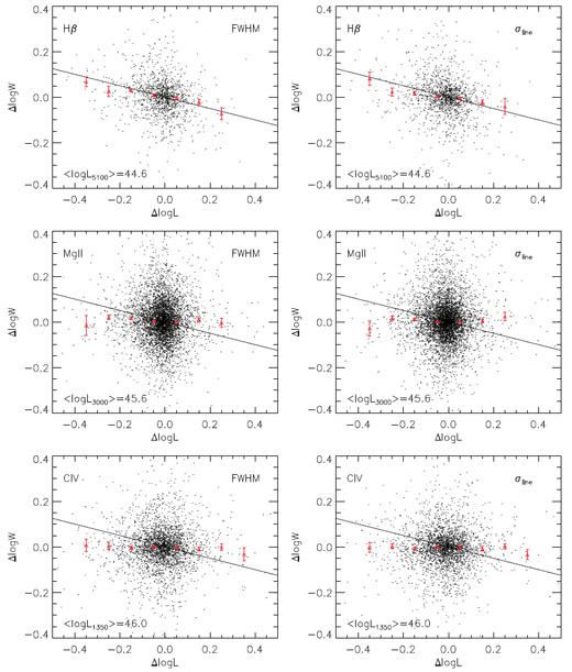Figure 1. A test of the virial assumption using two-epoch spectroscopy from SDSS for H (upper), Mg II (middle) and C IV (bottom). Plotted here are the changes in line width as a function of changes in continuum luminosity (L5100, L3000, and L1350 for H, Mg II, and C IV, respectively) between the two epochs. The left column is for FWHM and the right column is for line. The dots are for all objects with measurement S/N > 3 at both epochs for both L and W (not for log L and log W). These objects tend to cluster around zero values because the typical continuum and line variabilities of SDSS quasars are small. The red triangles are the median values in each log L bin, where the error bars indicate the uncertainty in the mean. A perfect virial relation would imply log W = -0.25 log L, as indicated by the solid line in each panel. Note that I have neglected the chromatic nature of quasar variability, which would predict an even steeper relation between log W and log L (see Section 3.1.1 for details). The low-redshift z 0.7 SDSS quasars with median luminosity < log (L5100 / erg s-1) > = 1044.6 show the expected virial relation between log L and log W, which is not the case for the high-luminosity SDSS quasars at z > 0.7 based on Mg II or C IV.

Another important point to make is that there is a well known fact that quasar spectra get harder (bluer) as they get brighter (e.g., Vanden Berk et al. 2004 and references therein). This means that the variability amplitude in the ionizing continuum should be larger than that at longer wavelengths (i.e., the observed continuum). Thus we should see a somewhat steeper slope in the line width change versus the (observed) continuum luminosity change plot for a single object (e.g., Peterson et al. 2002). This, however, would be in an even larger disagreement with the trends we see in Fig. 1.

3.1.2. The virial coefficient f

To relate the observed broad line width to the underlying virial velocity (e.g., Eqn. 2) requires the knowledge of the (emissivity weighted) geometry and kinematics of the BLR. In principle RM can provide such information, and determine the value of f from first principles. Unfortunately the current RM data are still not good enough for such purposes in general, although in a few cases alternative approaches have been invented lately to account for the effect of f in directly modeling the RM data using dynamical BLR models (e.g., Brewer et al. 2011, Pancoast et al. 2012). Early studies made assumptions about the geometry and structure of the BLR in deriving RM masses (e.g., Netzer 1990, Wandel et al. 1999, Kaspi et al. 2000) or SE virial masses (e.g., McLure & Dunlop 2004). Now the average value of f is mostly determined empirically by requiring that the RM masses are consistent with those predicted from the M_BH - _* relation of local inactive galaxies. Such an exercise was first done by Onken et al. (2004), who used 16 local AGNs with both RM measurements and stellar velocity dispersion measurements to derive < f > 1.4 if FWHM is used, or < f > 5.5 if _line is used. Later this was repeated with new RM data (e.g., Woo et al. 2010), who derived a similar value of < f > 5.2 (using _line).

However, in recent years it has become evident that the scaling relations between BH mass and bulge properties are not as simple as we thought: it appears that different types of galaxies follow somewhat different scaling relations, and the scatter seems to increase towards less massive systems (e.g., Hu 2008, Greene et al. 2008, Graham 2008, Graham & Li 2009, Hu 2009, Gültekin et al. 2009, Greene et al. 2010b, McConnell & Ma 2012 and references therein). Therefore, depending on the choice of the specific form of the M_BH - _* relation used and the types of galaxies hosting RM AGNs in the calibration, the derived average f value could vary significantly. For instance, Graham et al. (2011) derived a < f > value that is is only half of the values derived by Onken et al. (2004) and Woo et al. (2010). Park et al. (2012b) performed a detailed investigation on the effects of different regression methods and sample selection in determining the M_BH - _* relation and in turn the < f > value, and concluded that the latter is the primary cause for the discrepancy in the reported < f > values. Given the small sample sizes of RM AGNs with host property measurements and the uncertainties in the BH-host scaling relations in inactive galaxies, the uncertainty of < f > is still ~ a factor of 2 or more, and will remain one of the main obstacles to estimate accurate RM (or SE) BH masses in terms of the overall normalization. One may also expect that the actual f value is different in individual sources, either from the diversity in BLR structure or from orientation effects (since the line width only reflects the line-of-sight velocity, see Section 3.1.6). Thus using a constant f value in these RM masses and SE virial estimators introduces additional scatter in these mass estimates.

Perhaps a more serious concern is the assumption that the BH-host scaling relations are the same in active and inactive galaxies. While there is a clear correlation between bulge properties and the RM masses in RM AGNs (e.g., Bentz et al. 2009c), it could be offset from that for inactive galaxies if the actual < f > value is different. Such a scenario is plausible if the BH growth and host bulge formation are not always synchronized. The only way to tackle this problem is to infer f from directly constrained BLR geometry/kinematics with exquisite velocity-resolved RM data that map the line response (transfer function) in detail, and this must be done for a large number of AGNs to explore its diversity.

3.1.3. FWHM versus line dispersion

Both FWHM and _line are commonly used in SE virial mass estimates as the proxy for the virial velocity (when combined with the virial coefficient f). Both definitions have advantages and disadvantages. FWHM is a quantity that is easier to measure, less susceptible to noise in the wings and treatments of line blending than _line, while _line is less sensitive to the treatment of narrow line removal and peculiar line profiles. Overall FWHM is preferred over _line in terms of easiness of the measurement and repeatability. As _line measurements depend sensitively on data quality and different methods used (e.g., Denney et al. 2009b, Rafiee & Hall 2011a, Rafiee & Hall 2011b, Assef et al. 2011), the SE virial masses (e.g., Eqn. 4) based on _line could differ significantly for the same objects.

Physically one may argue _line is more trustworthy to use than FWHM, although the evidence to date is only suggestive. Collin et al. (2006) compared the virial products based on both _line and FWHM with those expected from the M_BH - _* relation, for 14 RM AGNs. All their line width measurements were based on the rms or mean spectra of the RM AGNs. They found that the average scale factor (i.e., the virial coefficient f) between virial products to the M_BH - _* masses depends on the shape of the line if FWHM is used, while it is more or less constant if _line is used. Based on this, they argue that _line is a better surrogate to use in estimating RM masses. Additionally, _line measured in rms spectra seems to follow the expected virial relation better than FWHM in some RM AGNs (e.g., Peterson et al. 2004), although such evidence is circumstantial.

It is important to note that for a given line, the ratio of FWHM to _line is not necessarily a constant (e.g., Collin et al. 2006, Peterson 2011 but cf., Decarli et al. 2008a), while a Gaussian line profile leads to FWHM / _line 2.35. For H, FWHM / _line seems to increase when the line width increases. This might be related to the Populations A and B sequences developed by Sulentic and collaborators (Sulentic et al. 2000a), which is an extension of earlier work on the correlation space of AGNs (the so-called "eigenvector 1", e.g., Boroson & Green 1992, Wang et al. 1996). A direct consequence is that there will be systematic differences in M_SE whether FWHM or _line is used for the same set of quasars, especially for objects with extreme line widths. In general a "tilt" between the FWHM and _line-based virial masses is expected (e.g., Rafiee & Hall 2011a, Rafiee & Hall 2011b). Currently directly measuring _line from single-epoch spectra is much more ambiguous and methodology-dependent than measuring FWHM. If one accepts that _line is a more robust virial velocity indicator, it is possible to convert the measured FWHM to _line using the relation found for high S/N data (e.g., Collin et al. 2006), or empirically determine the dependence of SE mass on FWHM (i.e., coefficient c in Eqn. 4) using RM masses as calibrators (e.g., Wang et al. 2009), which generally leads to values of c < 2.

The choice of line width indicators is still an open issue. It will be important to revisit the arguments in, e.g., Collin et al. (2006), using not only more but also better-quality RM data, as well as to investigate the behaviors of FWHM and _line (and perhaps alternative line width measures) for large quasar samples.

3.1.4. Broad line profiles

As briefly mentioned in Section 2.1, part of the reason that we are struggling with f and line width definitions is because of the simplifications of a single BLR size and using only one line profile characteristic to infer the underlying BLR velocity structure. If we have a decent understanding of the BLR dynamics and structure (geometry, kinematics, emissivity, ionization, etc.), then in principle we can solve the inverse problem of inferring the virial velocity from the broad line profile. Unfortunately, the detailed BLR properties are yet to be probed with velocity-resolved reverberation maps, and the solution of this inverse problem may not be unique (e.g., different BLR dynamics and structure may produce similar line profiles).

Nevertheless, there have been efforts to model the observed broad line profiles with simple BLR models. The best known example is the disk-emitter model (e.g., Chen et al. 1989, Eracleous & Halpern 1994, Eracleous et al. 1995), where a Keplerian disk with a turbulent broadening component is used to model the double-peaked broad line profile seen in ~ 10-15% radio-loud quasars (and several percent of radio-quite quasars). The line profile then can place constraints on certain geometrical parameters, such as the inclination of the disk, thus has relevance in the f value for individual objects (e.g., La Mura et al. 22009). Another example is using simple kinematic BLR models to explain the trend of the line shape parameter FWHM / _line as a function of line width (e.g., Kollatschny & Zetzl 2011, Kollatschny & Zetzl 2013), as mentioned earlier in Section 3.1.3. These authors found that a turbulent component broadened by a rotation component can explain the observed trend of line shape parameter, and their model provides conversions between the observed line width and the underlying virial (rotational) velocity. More complicated BLR models can be built (e.g., Goad et al. 2012), which has the potential to underpin a physical connection between the BLR structure and the observed broad line characteristics. While all these exercises are worth further investigations, it is important to build self-consistent models that are also verified with velocity-resolved RM.

3.1.5. Effects of host starlight and dust reddening

The luminosity that enters the R - L relation and the SE mass estimators (Eqn. 4) refers to the AGN luminosity. At low AGN luminosities, the contamination from host starlight to the 5100 Å luminosity can be significant. This motivated the alternative uses of Balmer line luminosities in Eqn. (4) (e.g., Greene & Ho 2005). Using line luminosity is also preferred for radio-loud objects where the continuum may be severely contaminated by the nonthermal emission from the jet (e.g., Wu et al. 2004). Bentz et al. (2006) and Bentz et al. (2009a) showed that properly accounting for the host starlight contamination at optical luminosities in RM AGNs leads to a slope in the R - L relation that is closer to the naive expectation from photoionization. Similarly, using host-corrected L₅₁₀₀ can lead to reduced scatter in the H - L₅₁₀₀ SE calibration against RM AGNs (e.g., Shen & Kelly 2012).

The average contribution of host starlight to L₅₁₀₀ has been quantified by Shen et al. (2011), using low-redshift SDSS quasars. They found that significant host contamination ( 20%) is present for logL_5100,total < 10^44.5 erg s^-1, and provided an empirical correction for this average contamination. Variations in host contribution could be substantial for individual objects though.

For UV luminosities (L₃₀₀₀, L₁₃₅₀ or L₁₄₅₀), the host contamination is usually negligible, although may be significant for rare objects with excessive ongoing star formation. A more serious concern, however, is that some quasars may be heavily reddened by dust internal or external to the host. The so-called "dust-reddened" quasars (e.g., Glikman et al. 2007) have UV luminosities significantly dust attenuated, and corrections are required to measure their intrinsic AGN luminosities. It is possible that optical quasar surveys (such as SDSS) are missing a significant population of dust-reddened quasars.

3.1.6. Effects of orientation and radiation pressure

If the BLR velocity distribution is not isotropic, orientation effects may affect the RM and SE mass estimates. Specific BLR geometry and kinematics, such as a flattened BLR where the orbits are confined to low latitudes, will lead to orientation-dependent line width. Some studies report a correlation between the broad line FWHM and the source orientation inferred from radio properties ⁵ (e.g., Wills & Browne 1986, Jarvis & McLure 2006), in favor of a flattened BLR geometry. Similar conclusions were achieved in Decarli et al. (2008a) based on somewhat different arguments. Since we use the average virial coefficient < f > in our RM and SE mass estimates, the true BH masses in individual sources may be over- or underestimated depending on the actual inclination of the BLR (e.g., Krolik 2001, Decarli et al. 2008a, Fine et al. 2011, Runnoe et al. 2013) ⁶. The distributions of broad line widths in bright quasars are typically log-normal, with dispersions of ~ 0.1-0.2 dex over ~ 5 magnitudes in luminosity (e.g., Shen et al. 2008a, Fine et al. 2008, Fine et al. 2010). A thin disk-like BLR geometry with a large range of inclination angles cannot account for such narrow distributions of line width, indicating either the inclination angle is limited to a narrow range for Type 1 objects, and/or there is a significant random velocity component (such as turbulent motion) of the BLR. This limits the scatter in BH mass estimates caused by orientation effects to be < 0.2-0.4 dex.

So far we have assumed that the dynamics of the BLR is dominated by the gravity of the central BH. The possible effects of radiation pressure, which also has a R^-2 dilution as gravity, on the BLR dynamics have been emphasized by, e.g., Krolik (2001). On average the possible radiation effects are eliminated in the empirical calibration of the < f > value (see Section 3.1.2), but neglecting such effects may introduce scatter in individual sources and luminosity-dependent trends. Most recently Marconi et al. (2008) modified the virial mass estimation by adding a luminosity term:

(6)

where the last term describes the effect of radiation pressure on the BLR dynamics with a free parameter g. By allowing this extra term, Marconi et al. (2008) re-calibrated the RM masses using the M_BH - _* relation, and the SE mass estimator using the new RM masses. This approach improves the rms scatter between single-epoch masses and RM masses, from ~ 0.4 dex to ~ 0.2 dex, and removes the slight systematic trend of the SE mass scatter with RM masses seen in Vestergaard & Peterson (2006). However, it is also possible that the reduction of scatter between the SE and RM masses is caused by the addition of fitting freedoms. Since the intrinsic errors on the RM masses are unlikely to be < 0.3 dex, optimizing the SE masses relative to RM masses to smaller scatter may lead to blown-up errors when apply the optimized scaling relation to other objects. It would be interesting to split the RM sample in Marconi et al. (2008) in half and use one half for calibration and the other half for prediction, and see if similar scatter can be achieved in both subsets. The relevance of radiation pressure is also questioned by Netzer (2009), who used large samples of Type 1 and Type 2 AGNs from the SDSS to show that the radiation-pressure corrected viral masses lead to inconsistent Eddington ratio distributions in Type 1s and Type 2s, even though the [O III] luminosity distribution is consistent in the two samples. However, Marconi et al. (2009) argues that the difference in the "observed" Eddington ratio distributions does not mean that radiation pressure is not important, rather it could result from a broad range of column densities which are not properly described by single values of parameters in the radiation-pressure-corrected mass formula. These studies then revealed that using the simple corrected formula as provided in Marconi et al. (2008) does not provide a satisfactory recipe to account for radiation pressure in RM or SE mass estimates, and the relevance of radiation pressure and a practical method to correct for its effect are therefore still under active investigations (e.g., Netzer & Marziani 2010).

3.1.7. Comparison among different line estimators

There are both low-ionization and high-ionization broad lines in the restframe UV to near-infrared of the quasar spectrum. Despite different ionization potential and probably different BLR structure, several of them have been adopted as SE virial mass estimators. The most frequently used line-luminosity pairs include strong Balmer lines (H and H) with L₅₁₀₀ or L_{H, H}, Mg II with L₃₀₀₀, and C IV with L₁₃₅₀ or L₁₄₅₀. Hydrogen Paschen lines in the near-IR can also be used if such near-IR spectroscopy exists.

There have been SE calibrations upon specific lines against RM masses, or against SE masses based on another line. Comparisons between different SE line estimators using various quasar samples are often made in the literature: some claim consistency, while others report discrepancy. As emphasized in Shen et al. (2008a), it is important to use a consistent method in measuring luminosity and line width with that used for the calibrations if one wants to make a fair comparison using external samples. Failure to do so may lead to unreliable conclusions (e.g., Dietrich & Hamann 2004).

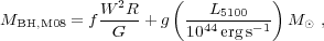
The continuum luminosities at different wavelengths and several line luminosities are all correlated with each other, with different levels of scatter. Fig. 2 shows some correlations between different continuum luminosities using the spectral measurements of SDSS quasars from Shen et al. (2011). To compare L₁₃₅₀ and L₅₁₀₀ directly, one needs either UV+optical or optical+near-IR to cover both restframe wavelengths. Fig. 2 (left) shows such a comparison from a recent sample of quasars with optical spectra from SDSS and near-IR spectra from Shen & Liu (2012), which probes a higher luminosity range L₅₁₀₀ > 10^45.4 erg s^-1 than the SDSS sample. Correlations between these luminosities are still seen at the high-luminosity end. For the SDSS quasar population, different luminosities correlate with each other well, but this may be somewhat affected by the optical target selection of SDSS quasars that may preferentially miss dust-reddened quasars (see Section 3.1.5). In other words, the intrinsic dispersion in the UV-optical SED may be larger for the general quasar population. For instance, Assef et al. (2011) found a much larger dispersion in the L₁₃₅₀ / L₅₁₀₀ ratio for a gravitationally lensed quasar sample, which is selected differently from the SDSS. This large dispersion in the L₁₃₅₀ / L₅₁₀₀ ratio will lead to more scatter between the H and C IV based SE masses.

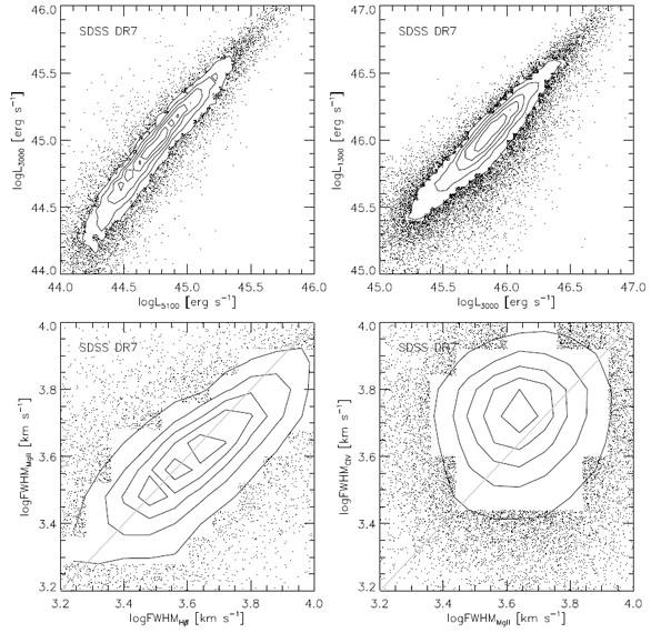Figure 2. Comparisons between different continuum luminosities and line FWHMs, using SDSS quasar spectra that cover two lines. Shown here are the local point density contours. Measurements are from Shen et al 2011. The upper panels show the correlations between continuum luminosities, and the bottom panels show the correlations between line FWHMs. While the Mg II FWHM correlates with H FWHM reasonably well, the correlation between the C IV FWHM and Mg II FWHM is poor (also see, e.g., Shen et al 2008a, Fine et al 2008, 2010).

It is also important to compare the widths of different lines. Since H is the most studied line in reverberation mapping and the R - L relation was measured using BLR radius for H (e.g., Kaspi et al. 2000, Kaspi et al. 2005, Bentz et al. 2009a), it is reasonable to argue that the SE mass estimators based on the Balmer lines are the most reliable ones. The width of the broad H is well correlated with that of the broad H and therefore it provides a good substitution in the absence of H (e.g., Greene & Ho 2005). The widths of Mg II are found to correlate well with those of the Balmer lines (e.g., see Fig. 2 for a comparison based on SDSS quasars Salviander et al. 2007, McGill et al. 2008, Shen et al. 2008a, Shen et al. 2011, Wang et al. 2009, Vestergaard et al. 2011, Shen & Liu 2012). But such a correlation may not be linear: despite different methods to measure line widths, most recent studies favor a slope shallower than unity in the correlation between the two FWHMs (e.g., see Fig. 2). Given this correlation it is practical to use the Mg II width as a surrogate for H width in a Mg II-based SE mass estimators, and some recent Mg II calibrations can be found in, e.g., Vestergaard & Osmer (2009), Shen & Liu (2012), Trakhtenbrot & Netzer (2012). However, one intriguing feature regarding the Mg II line is that the distribution of its line widths seem to have small dispersions in large quasar samples (e.g., Shen et al. 2008a, Fine et al. 2008). It appears as if the Mg II varies at a less extent compared with H (cf., Woo 2008 and references therein). It is also recently argued that for a small fraction of quasars (~ 10%) in the NLS1 regime (e.g., small H FWHM and strong FeII emission), Mg II may have a blueshifted, non-virial component, and an overall larger FWHM than H, that will bias the virial mass estimate (e.g., Marziani et al. 2013). This is consistent with the general trend found between Mg II and H FWHMs using SDSS quasars (e.g., Wang et al. 2009, Shen et al. 2011, Vestergaard et al. 2011), and may be connected to the disk wind scenario for C IV discussed below.

The correlation between H (or MII) and C IV widths is more controversial. While some claim that these two do not correlate well (e.g., Bachev et al. 2004, Baskin & Laor 2005, Netzer et al. 2007, Shen et al. 2008a, Fine et al. 2010, Shen & Liu 2012, Trakhtenbrot & Netzer 2012), others claim there is a significant correlation (e.g., Vestergaard & Peterson 2006, Assef et al. 2011). Fig. 3 (right) shows a compilation of C IV and H FWHMs from the literature, which are derived for quasars in different luminosities and redshift ranges. Only the low-luminosity (and low-z) RM sample in Vestergaard & Peterson (2006) shows a significant correlation. It is often argued that sufficient data quality is needed to secure the C IV FWHM measurements, although measurement errors are unlikely to account for all the scatter seen in the comparison between C IV and H FWHMs - the correlation between the two is still considerably poorer than that between Mg II and H FWHMs for the samples in Fig. 3 when restricted to high-quality data. Shen & Liu (2012) suggested that the reported strong correlation between C IV and H FWHMs is probably caused by the small sample statistics, or only valid for low-luminosity objects.

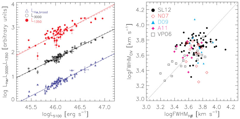Figure 3. Left: correlations between different luminosities using the quasar sample in Shen & Liu (2012), which covers all four lines (C IV, Mg II, H, H) in the same object, for the high-luminosity regime L5100 > 1045.4 erg s-1}. The solid lines are the bisector linear regression results using the BCES estimator (e.g., Akritas & Bershady 1996), and the dashed lines indicate a linear correlation of unity slope. Right: comparison between C IV FWHM and H FWHM using different samples from the literature [Shen & Liu (2012, 60 objects; SL12), Assef et al (2011, 9 objects; A11), Vestergaard & Peterson (2006, 21 objects; VP06), Netzer et al. (2007, 15 objects; N07), and Dietrich et al. (2009, 9 objects; D09)]. Only for the low-redshift and low-luminosity VP06 sample is there a significant correlation between the two FWHMs.

The high-ionization C IV line also differs from low-ionization lines such as Mg II and the Balmer lines in many ways (for a review, see Sulentic et al. 2000b). Most notably it shows a prominent blueshift (typically hundreds, up to thousands of km s^-1) with respect to the low-ionization lines (e.g., Gaskell 1982, Tytler & Fan 1992, Richards et al. 2002), which becomes more prominent when luminosity increases. There is also a systemic trend (albeit with large scatter) of increasing C IV FWHM and line asymmetry when the C IV blueshift increases, a trend not present for low-ionization lines (e.g., Shen et al. 2008a, Shen et al. 2011). The C IV blueshift is predominantly believed to be an indication of outflows in some form, and integrated in the disk-wind framework discussed below (but see Gaskell 2009 for a different interpretation). These properties of C IV motivated the idea that C IV is likely more affected by a non-virial component than low-ionization lines (e.g., Shen et al. 2008a), probably from a radiatively-driven (and/or MHD-driven) accretion disk wind (e.g., Konigl & Kartje 1994, Murray et al. 1995, Proga et al. 2000, Everett 2005), especially for high-luminosity objects. A generic two-component model for the C IV emission is then implied (e.g., Collin-Souffrin et al. 1988, Richards et al. 2011, Wang et al. 2011). A similar argument is proposed by Denney (2012) based on the C IV RM data of local AGNs, where she finds that there is a component of the C IV line profile that does not reverberate, which is likely associated with the disk wind (although alternative interpretations exist). This may also explain the poorer correlation between C IV width and H (or Mg II) width for more luminous quasars, where the wind component is stronger (see further discussion in Section 3.1.9). Therefore C IV is likely a biased virial mass estimator (e.g., Baskin & Laor 2005, Sulentic et al. 2007, Netzer et al. 2007, Shen et al. 2008a, Marziani & Sulentic 2012 and references therein).

Although in principle certain properties of C IV (such as line shape parameters) can be used to infer the C IV blueshift and then correct for the C IV-based SE mass, such corrections are difficult in practice given the large scatter in these trends and typical spectral quality. Proponents on the usage of C IV line often emphasize the need for good-quality spectra and proper measurements of the line width. But the fact is C IV is indeed more problematic than the other lines, and there is no immediate way to improve the C IV estimator for high-redshift quasars, although some recent works are showing some promising trends that may be used to improve the C IV estimator (e.g., Denney 2012).

There have also been proposals for using the C III], Al III, or Si III] lines in replacement of C IV (e.g., Greene et al. 2010a, Marziani & Sulentic 2012). Shen & Liu (2012) found that the FWHMs of C IV and C III] are correlated with each other, and hence C III] may not be a good line either (also see Ho et al. 2012). On the other hand, Al III and Si III] are more difficult to measure given their relative weakness compared to C IV and C III] as well as their blend nature, hence are not practical for large samples of quasars. Another possible line to use is Ly. Although Ly is more severely affected by absorption, intrinsically it may behave similarly as the Balmer lines. Such an investigation is ongoing.

To summarize, currently the most reliable lines to use are the Balmer lines, although this conclusion is largely based on the fact that these are the most studied and best understood lines, and does not mean there is no problem with them. Mg II can be used in the absence of the Balmer lines, although the lack of RM data for Mg II poses some uneasiness in its usage as a SE estimator. C IV has local RM data (though not enough to derive a R - L relation on its own), but the application of C IV to high-redshift and/or high-luminosity quasars should proceed with caution. In light of the potential problems with C IV, efforts have been underway to acquire near-IR spectroscopy to study the high-z quasar BH masses using Mg II and Balmer lines (e.g., Shemmer et al. 2004, Netzer et al. 2007, Marziani et al. 2009, Dietrich et al. 2009, Greene et al. 2010a, Trakhtenbrot et al. 2011, Assef et al. 2011, Shen & Liu 2012, Ho et al. 2012, Matsuoka et al. 2013).

3.1.8. Effects of AGN variability on SE masses

Quasars and AGNs vary on a wide range of timescales. It is variability that made reverberation mapping possible in the first place. One might be concerned that the SE masses may subject to changes due to quasar variability. Several studies have shown, using multi-epoch spectra of quasars, that the scatter due to luminosity changes (and possibly corresponding changes in line width) does not introduce significant ( 0.1 dex) scatter to the SE masses (e.g., Wilhite et al. 2007, Denney et al. 2009b, Park et al. 2012a). This is expected, since the average luminosity variability amplitude of quasars is only ~ 0.1-0.2 magnitude over month-to-year timescales (e.g., Sesar et al. 2007, MacLeod et al. 2010, MacLeod et al. 2012), thus the difference in SE masses from multi-epochs will be dominated by measurement errors (in particular those on line widths).

However it is legitimate to consider the consequence of uncorrelated stochastic variations between line width and luminosity on SE masses, whether or not such uncorrelated variations are due to actual physical effects, or due to improper measurements of the continuum luminosity and line widths. Examples are already given in Section 3.1.1, and more detailed discussion will be provided in Section 3.3.

3.1.9. Limitations of the RM AGN sample

Last but not least, the current RM sample is by no means representative of the general quasar/AGN population. It is a highly heterogeneous sample that poorly samples the high-luminosity regime of quasars, and most objects are at z < 0.3. This alone calls into question the reliability of extrapolations of locally-calibrated SE relations against these RM AGNs to high-z and/or high-luminosity quasars.

The distribution of the RM AGNs in the spectral parameter space of quasars is also highly biased relative to the general population. Richards et al. (2011) developed (building on earlier ideas by, e.g., Collin-Souffrin et al. 1988, Murray et al. 1995, Proga et al. 2000, Elvis 2000, Leighly & Moore 2004, 1492004Leighly ) a generic picture of two-component BLR structure for C IV, composed of a virial component, and a non-virial wind component which is filtering the ionizing continuum from the inner accretion disk. This generic picture is able to explain, phenomenologically, many characteristics of the continuum and C IV line properties, such as the C IV blueshift and the Baldwin effect (i.e., the anti-correlation between C IV equivalent width and adjacent continuum luminosity, Baldwin 1977). Fig. 4 shows the distribution of RM objects in the parameter space of C IV spectral properties, where most RM AGNs occupy the regime dominated by the virial component. Part of this is driven by luminosity, since more luminous quasars have on average larger C IV blueshift (Section 3.1.7). It will be important to explore this under-represented regime with C IV RM at high-redshift, which has just begun (e.g., Kaspi et al. 2007). Although this is an immediate concern for C IV, Richards et al. (2011) made a fair argument that the BLR properties for H and Mg II may also be biased in the RM sample relative to all quasars, if the non-virial wind component is also affecting the BLR of H and Mg II by filtering the ionizing continuum.

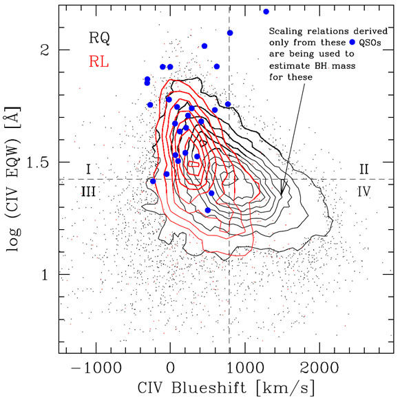Figure 4. An updated version of Fig. 18 in Richards et al (2011), showing the biased distribution of the local RM AGNs in the parameter space for C IV (blueshift relative to Mg II versus the rest equivalent width). The contours and dots are 1.5 z 2.2 SDSS quasars, and the blue filled circles are RM AGNs. The black and red contours show the results for radio-quiet and radio-loud populations respectively. Most of the RM AGNs occupy quadrant I, where the C IV line is dominated by the virial component in the two-component picture in Richards et al (2011). In this picture, quadrant IV is for C IV lines dominated by the non-virial wind component. The average quasar luminosity increases from quadrant I to quadrant IV. Figure courtesy of G. Richards.

To date most of the RM lag measurements are for H, and lag measurements are either lacking for Mg II (but see Metzroth et al. 2006, Woo 2008 and references therein, for Mg II RM attempts and tentative results) or insufficient for C IV to derive a direct R - L relation based on these two UV lines. The total number of RM AGNs is also small, ~ 50, not enough to probe the diversity in BLR structure and other general quasar properties. The current sample size and inhomogeneity of RM AGNs pose another major obstacle to develop precise BH mass estimators based on RM and its extension, SE virial methods.

3.2. Practical Concerns

3.2.1. How to measure the continuum luminosity and line widths

Usually the continuum and line properties are measured either directly from the spectrum, or derived from ² fits to the spectrum with some functional forms for the continuum and for the lines. Arguably functional fits are better suited for spectroscopic samples with moderate to low spectral quality. As briefly mentioned earlier (Section 3.1.7), it is essential to measure the continuum and line width properly when using the existing SE calibrations. Different methods sometimes do yield systematically different results, in particular for the line width measurements. Some studies fit the broad lines with a single component (e.g., McLure & Dunlop 2004), while others use multiple components to fit the broad line. But if one wants to use the calibration in, e.g., McLure & Dunlop (2004), then it is better to be consistent with their fitting method. Some comparisons between the broad line widths from different fitting recipes can be made using the catalog provided in Shen et al. (2011). Take H for example, since this broad line is not always a single Gaussian or Lorentzian, the line widths from the single-component and multiple-component fit could differ significantly in some cases.

The detailed description of spectral fitting procedure can be found in many papers (e.g., McLure & Dunlop 2004, Greene & Ho 2005, Shen et al. 2008a, Shen et al. 2011, Shen & Liu 2012). In short, the spectrum is first fit with a power-law plus an iron emission template ⁷ in several spectral windows free of major broad lines. The best-fit "pseudo-continuum" is then subtracted from the original spectrum, leaving the emission line spectrum. The broad line region is then fit with a mixture of functions (such as multiple Gaussians or Gauss-Hermite polynomials). The continuum luminosity and line width are then extracted from the best-fit model. The measurement errors from the multiple component fits are often estimated using some Monte Carlo methods (e.g., Shen et al. 2011, Shen & Liu 2012): mock spectra are generated either by adding noise to the original spectrum, or by adding "scrambled" residuals from the data minus best-fit model back to the model. The mock spectra are then fit with the same fitting procedure, and the formal errors are estimated from the distributions of the measured quantity from the mocks. This mock-based error estimation approach takes into account both the noise of the spectrum and ambiguities in decomposing different components in the fits.

Below are some additional notes regarding continuum and line measurements.

• Narrow line subtraction Since the narrow line region (NLR) dynamics is not dominated by the central BH gravity, we want to subtract strong narrow line component before we measure the broad line width from the spectrum. This is particularly important for FWHM measurements, while for _line the effects of narrow lines are less important. For H and H, reliable constraints on the velocity and width of the narrow components can be obtained from the adjacent narrow lines such as [O III] 4959,5007 and [S II] 6717,6731. For Mg II and C IV, this is not so simple mainly for two reasons: 1) there are usually no adjacent strong narrow lines such as [O III] to provide constraints on the narrow line component; and even if [O III] can be covered in other wavelengths there is no guarantee the NLR properties are the same for [O III] and for Mg II / C IV. 2) Although some quasars do show evidence of narrow component Mg II and C IV, it is unclear if this applies to the general quasar population. Shen & Liu (2012) found that for the 60 high-luminosity (L₅₁₀₀ > 10^45.4 erg s^-1) quasars in their sample with optical and near-IR spectroscopy covering C IV to [O III], the contribution of the narrow line component to C IV is too small to affect the estimated broad C IV FWHM significantly. However, for less luminous objects, the relative importance of the narrow line component to C IV might be larger (e.g., Bachev et al. 2004, Sulentic et al. 2007).

• Remedy for absorption Sometimes there are absorption features superposed on the spectrum, which is most relevant for C IV, and then Mg II. Not accounting for these absorption features will bias the continuum and line measurements. While for narrow or moderately-broad absorption troughs, manual or automatic treatments can greatly minimize their effects (e.g., Shen et al. 2011), there is no easy way to fit objects that are heavily absorbed (such as broad absorption line quasars).

• Effects of low signal-to-noise ratio (S/N) The quality of the continuum luminosity and line width measurements decreases as the quality of the spectrum degrades. In addition to increased measurement errors, low S/N data may also lead to biases in the spectral measurements. Denney et al. (2009b) performed a detailed investigation on the effects of S/N on the measured H line width using many single-epoch spectra of two RM AGNs (NGC 5548 and PG 1229+204). They tested both direct measurements and Gauss-Hermite polynomial fits to the spectrum, and found that the best-fit line width is systematically underestimated at low S/N for both direct measurements and functional fits. The only exception is that their Gauss-Hermite fits to degraded NGC 5548 spectra tend to overestimate the FWHM at lower S/N. However, this is mainly caused by the fact that the Gauss-Hermite model is often unable to accurately fit the complex H line profile of NGC 5548. Using multiple-Gaussian model fits, and for a much larger sample of SDSS quasars, Shen et al. (2011) also investigated the effects of S/N on the model fits by artificially degrading high S/N spectra (see their Figs. 5-8). They found that the exact magnitude of the bias depends on the line profile as well as the strength of the line. The continuum is usually unbiased as S/N decreases. The FWHMs and equivalent widths (EWs) are biased by less than ± 20% for high-EW objects as S/N is reduced to as low as ~ 3/pixel. For low-EW objects, the FWHMs and EWs are biased low/high by > 20% for S/N 5/pixel. But the direction of the bias in FWHM is not always underestimation.

3.3. Consequences of the Uncertainties in SE Mass Estimates

Given the many physical and practical concerns discussed in Sections 3.1 and 3.2, one immediately realizes that these mass estimates, especially those SE mass estimates, should be interpreted with great caution. Almost everyone acknowledges the large uncertainties associated with these mass estimates, but only very few are taking these uncertainties seriously. Since at present there is no way to know whether or not the extrapolation of these SE methods to high-z and/or high-luminosity quasars introduces significant biases, let us assume naively that these SE estimators provide unbiased mass estimates in the average sense, and focus on the statistical uncertainties (scatter) of these estimators.

In mathematical terms, we have:

(7)

where m_e ≡ logM_BH,SE is the SE mass estimate, m ≡ M_BH is the true BH mass, and G(µ, ) is a Gaussian random deviate with mean µ and dispersion . I use x | y to denote a random value of x at fixed y drawn from the conditional probability distribution p(x|y). Eqn. (7) thus means that the distribution of SE masses given true BH mass, p₀(m_e | m), is a lognormal with mean equal to m and dispersion _SE. It is then clear that this equation stipulates our assumption that the SE mass is on average an unbiased estimate of the true mass, but with a statistical scatter of _SE ~ 0.5 (dex), i.e., the formal uncertainty of SE masses.

3.3.1.   The Malmquist-type bias (Eddington bias)

Now let us assume that we have a mass-selected sample of objects with known true BH masses, and "observed" masses based on the SE estimators. By "mass-selected" I mean there is no selection bias caused by a flux (or luminosity) threshold – all BHs are observed regardless of their luminosity. If we further assume that the distribution of true BH masses in this sample is bottom-heavy, then a statistical bias in the SE masses naturally arises from the errors of SE masses (e.g., Shen et al. 2008a, Kelly et al. 2009a, Shen & Kelly 2010, Kelly et al. 2010), because there are more intrinsically lower-mass objects scattering into a SE mass bin due to errors than do intrinsically higher-mass objects. This statistical bias can be shown analytically assuming simple analytical forms of the distribution of true BH masses. Suppose the underlying true mass distribution is a power-law, dN / dM_BH M_BH^M, then Bayes's theorem tells us the distribution of true BH masses at given SE mass is (recall p₀(m_e|m) is the conditional probability distribution of m_e given m):

(8)

Thus the expectation value of true mass at given SE mass is:

(9)

Therefore for bottom-heavy (_M < 0) true mass distributions, the average true mass at given SE mass is smaller by -ln(10) _{M SE}² dex than the SE mass. This has an important consequence that the quasar black hole mass function (BHMF) constructed using SE virial masses will be severely overestimated at the high-mass end (e.g., Kelly et al. 2009a, Kelly et al. 2010, Shen & Kelly 2012).

This statistical bias due to the uncertainty in the mass estimates and a non-flat true mass distribution is formally known as the Eddington bias (Eddington 1913). Historically this has also been referred to as the Malmquist bias in studies involving distance estimates (e.g., Lynden-Bell et al. 1988), which bear some resemblance to the familiar Malmquist bias in magnitude-limited samples (e.g., Malmquist 1922). For this reason, this bias was called the "Malmquist" or "Malmquist-type" bias in Shen et al. (2008a) and Shen & Kelly (2010), and I adopted this name here as well. Perhaps a better name for this class of biases is the "Bayes correction", which then also applies to the generalization of statistical biases caused by threshold data and correlation scatter (or measurement errors). The luminosity-dependent bias discussed next, and the Lauer et al. bias (Lauer et al. 2007) discussed in Section 4.3, can also be described by this name.

3.3.2.   Luminosity-dependent bias in SE virial BH masses

Now let us take one step further, and consider the conditional probability distribution of m_e at fixed true mass m and fixed luminosity l ≡ logL, p(m_e|m, l). If the SE mass distribution at given true mass is independent on luminosity, then we have p(m_e|m, l) = p(m_e|m). This means that the SE mass is always unbiased in the mean regardless of luminosity. However, one may consider such a situation where p(m_e|m, l) ≠ p(m_e|m), which means the distribution of SE masses will be modified once one limits on luminosity. This is an important issue, since essentially all statistical quasar samples are flux-limited samples (except for heterogeneous samples, such as the local RM AGN sample), and frequently the SE mass distribution in finite luminosity bins is measured and interpreted.

Below I will explore this possibility and its consequences in detail. To help the reader understand these issues, here is an outline of the discussion that follows: 1) I will first formulate the basic equations to understand the (mathematical) origin of the uncertainty in SE mass, _SE; 2) I will then provide physical considerations to justify this formulation; 3) The conditional probability distribution of SE mass at fixed true mass and luminosity p(m_e|m, l) is then derived, and I demonstrate the two most important consequences: the luminosity-dependent bias, and the narrower distribution of SE masses at fixed true mass and luminosity than the SE mass uncertainty _SE; 4) I then discuss current observational constraints on the luminosity-dependent bias and demonstrate its effect using a simulated flux-limited quasar sample.

1) Understanding the origin of the uncertainty _SE in SE masses

I will use Gaussians (lognormal) to describe most distributions and neglect higher-order moments, mainly because the current precision and our understanding of SE masses are not sufficient for more sophisticated modeling. Assuming the distributions of luminosity and line width at given true mass m both follow lognormal distributions, we can write such distributions as

(10)

where notations are the same as in Eqn. (7), w ≡ logW, and <>_m indicates the expectation value at m. The dispersions in luminosity and line width at this fixed true mass should be understood as due to both variations in single objects (i.e., variability) and object-by-object variance. The SE mass estimated using l and w are then (e.g., Eqn. 4):

(11)

where the last term "constant" absorbs coefficient a and other constants from SE mass calibrations. Now let us consider the following two scenarios:

• A. In the ideal case where the SE method gives a perfect mass estimate, we have

  (12)

  i.e., the deviations in luminosity and line width from their mean values at given true mass are perfectly correlated. The resulting m_e distribution thus peaks at m with zero width, i.e., m_e|m = m = b < l >_m + c < w >_m + constant.

• B. In the realistic case, certain amount of the deviations in l and w from their mean values are uncorrelated with each other (either intrinsic or due to measurement errors). Without loss of generality, we can rewrite Eqn. (10) as

  (13)

  where the total dispersions in the distributions of l and w are

  (14)

  Eqn. (13) stipulates that some portions of the dispersions in l and w, described by _corr, are correlated and do not contribute to the dispersion (scatter) of m_e at m. On the other hand, the remaining dispersions in l ('_l) and in w ('_w) are stochastic terms, and they combine to cause the dispersion of m_e at m:

  (15)

  where

  (16)

  is the formal uncertainty in SE mass, i.e., the scatter in m_e at given true mass m.

Eqn. (13) through (16) provide a general description of SE mass error budget from luminosity and line width, and form the basis of the following discussion. From now on I will only consider the realistic case B.

2) Physical considerations on the variances '_l, '_w and _corr

Most of the studies to date have implicitly assumed '_l = 0 in Eqn. (13), with the few exceptions in e.g., Shen et al. (2008a), Shen & Kelly (2010) and Shen & Kelly (2012). '_l = 0 imposes a strong requirement that all the variations in luminosity are compensated by line width such that the uncertainty in SE masses now completely comes from the '_w part in line width dispersion. While this is what we hope for the SE method, there are physical and practical reasons to expect a non-zero '_l, as discussed in, e.g., Shen & Kelly (2012). Specifically we have the following considerations:

(a) the stochastic continuum luminosity variation and response of the BLR (hence the response in line width) are not synchronized, as resulting from the time lag in the reverberation of the BLR. The rms continuum variability on timescales of the BLR light-cross time is ~ 0.05 dex using the ensemble structure function in, e.g., MacLeod et al. (2010);

(b) even with the same true mass, individual quasars have different BLR properties, and presumably the measured optical-UV continuum luminosity is not as tightly connected to the BLR as the ionizing luminosity. Both will lead to stochastic deviations of luminosity and line width from the perfect correlation (source-by-source variation in the virial coefficient f, scatter in the R - L relation, etc.). The level of this luminosity stochasticity is unknown but is at least 0.2-0.3 dex given the scatter in the R - L relation alone, and thus it is a major contributor to '_l;

(c) although not explicitly specified in Eqn. (13), there are uncorrelated measurement errors in luminosity and line width; typical measurement error in luminosity for SDSS spectra (with S/N ~ 5-10/pixel, e.g., see fig. 4 of Shen et al. 2011) is ~ 0.02 dex (statistical only), but increases rapidly at low S/N;

(d) and finally, what we measure as line width does not perfectly trace the virial velocity. This is a concern for essentially all three lines, and for both of the two common definitions of line width (FWHM and _line). Two particular concerns arise. First, single-epoch spectra do not provide a line width that describes the reverberating part of the line only, thus some portion of the line width may not respond to luminosity variations. Second, if a line is affected by a non-virial component (say, C IV for instance), and if this component strengthens and widens when luminosity increases, the total line width would not response to the luminosity variation as expected. As in (b), this contribution to the uncompensated (by line width) luminosity variance '_l is unknown, but could be as significant as in (b).

One extreme of (d) would be that line width has nothing to do with the virial velocity except for providing a mean value in the calibrations of Eqn. (4), as suggested by Croom (2011), i.e., _corr = 0. In this case while the average SE masses are unbiased by calibration, the luminosity-dependent SE mass bias at given true mass is maximum (see below). Note that this _corr=0 case was already considered in Shen et al. (2008a) and Shen & Kelly (2010) when demonstrating the luminosity-dependent bias, and is only a special case of the above generalized formalism.

On the other hand, _corr > 0 would mean that line width does respond to luminosity variations to some extent, justifying the inclusion of line width in Eqn. (4). This was indeed seen at least for some local, low-luminosity objects, although not so much for the high-luminosity SDSS sample, based on the tests described in Section 3.1.1; additional evidence is provided in, e.g., Kelly & Bechtold (2007) and Assef et al. (2012), again for the low-luminosity RM AGN sample. Therefore, the most realistic scenario is that at fixed true mass, some portions of the dispersions in luminosity (or equivalently, Eddington ratio) and in line width are correlated with each other, and they cancel out in the calculation of SE masses; the remaining portions of the dispersions in l and w are stochastic in nature and they combine to contribute to the SE mass uncertainty (as in Eqn. 16). In other words, we expect '_l > 0, '_w > 0, and _corr > 0. For simplicity I take constant values for these scatters in the following discussion, but it is possible that they depend on true BH mass.

3) The distribution of SE mass at fixed true mass and luminosity p(m_e|m,l)

Now that we have formulated the distributions of l, w and m_e at fixed m (e.g., Eqns. 11 and 13), we can derive the conditional probability distribution of m_e at fixed m and l, p(m_e|m,l). It is straightforward to show ⁸ (again using Bayes's theorem) that this distribution is also a Gaussian distribution, with mean and dispersion:

(17)

Therefore we can generate the distribution of m_e at fixed m and l as:

(18)

where (using Eqns. 14 and 16)

(19)

Physically _ml is the dispersion of SE mass at fixed true mass and fixed luminosity. The parameter denotes the magnitude (slope) of the luminosity-dependent bias, and we have ⁹ 0 < < b, where the lower and upper boundaries correspond to the two extreme cases '_l = 0 and _corr = 0. A larger means a stronger luminosity-dependent bias. Given the values of '_l, '_w and _corr, and a SE calibration (b and c), all other quantities can be derived using Eqns. (14) - (19).

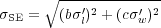
Fig. 5 shows a demonstration with '_l = 0.6, _corr = 0.1, '_w = 0.15, b = 0.5 and c = 2. In this example we have = 0.49, _SE = 0.42, and _ml = 0.3. The left two panels show the distributions of luminosity and line width at fixed true mass, from the stochastic term ('_l, '_w), the correlated term (_corr) and the total dispersion (_l, _w). The right panel shows the distributions of SE masses at this fixed true mass for all luminosities (black dotted line) and for fixed luminosities (green and red dotted lines). The distributions of SE masses at fixed luminosity are both narrower and biased compared with the distribution without luminosity constraint.

Figure 5. Simulated distributions of l (left), w (middle), and me (right) at fixed true mass m, following the description in Section 3.3.2 (e.g., see Eqns. 13-19). The example shown here assumes b = 0.5, c = 2 in Eqn. (13), e.g., the typical values for SE mass estimators. Left: The distribution of luminosity l ≡ log L. The black dotted line indicates the dispersion in 'l = 0.6, the cyan dashed line indicates the dispersion in corr = 0.1, and the black solid line indicates the total dispersion in l = ('l2 + corr2)1/2 (which essentially overlaps with the dotted line given that l is dominated by 'l). Middle: The distribution of line width w ≡ log W. The black dotted line indicates the dispersion in 'w = 0.15, the cyan dashed line indicates the dispersion in -corr b/c (i.e., the part that correlates with luminosity), and the black solid line indicates the total dispersion in w = ['w2 + (corr b/c)]1/2. Again the solid line and the dotted line are almost on top of each other. Right: The distribution of SE mass me ≡ log MSE. The black dotted line indicates the total dispersion of me at fixed m, SE = [(b'l)2 + (c'w)2]1/2 = 0.42. The green (red) dotted line indicates the distribution of me at fixed m and fixed l = <l> - 0.5 (<l> + 0.5), which is a Gaussian described by Eqns. (18)-(19). In this example most of the dispersions in luminosity and line width are uncorrelated with each other, leading to a large uncertainty in SE masses SE = 0.42 dex. The inferred luminosity-dependent bias has a slope of = 0.49. The dispersion of me at fixed luminosity is only ml = 0.3 dex (Eqn. 19), much smaller than the uncertainty in SE masses, SE.

• At fixed true mass m, the SE mass m_e is over-/underestimated when luminosity l is higher/lower than the average value at fixed m. This is the "luminosity-dependent bias" first introduced in Shen et al. (2008a) and subsequently developed in Shen & Kelly (2010) and Shen & Kelly (2012). The magnitude of this bias, determined by , depends on how much of the dispersion in luminosity at fixed true mass is stochastic with respect to line width (i.e., not compensated by responses in w).

• Secondly, the variance in SE masses at fixed true mass and fixed luminosity, _ml², is generally smaller than the uncertainty of SE masses, _SE², by an amount of ( _l)². A simple way to understand this is that the uncertainty (variance) of SE mass at fixed true mass comes from the stochastic variance terms in both luminosity and line width. Therefore when one reduces the variance in either luminosity or line width by fixing either variable, the variance in SE mass is also reduced. This has important consequences in interpreting the observed distribution of SE masses for quasars in flux-limited samples or in narrow luminosity bins. One cannot simply argue (as did in, e.g., Kollmeier et al. 2006, Steinhardt & Elvis 2010b) that the uncertainty in SE masses is small because the distribution of SE masses for samples with restricted luminosity ranges is narrow. The example shown in Fig. 5 clearly demonstrates that one can easily get a much narrower SE mass distribution at fixed true mass and luminosity, than the nominal SE mass uncertainty _SE. On the other hand, if enforcing '_l = 0, then _SE = c '_w < c _w, and there will be tension between the observed narrow distribution in line width (e.g., Shen et al. 2008a, Fine et al. 2008), which indicates _w 0.15 dex for Mg II, and the expectation that _SE >0.3 dex.

4) Observational constraints on the luminosity-dependent bias

The exact value of is difficult to determine observationally, although some rough estimates can be made based on monitoring data of single objects, or samples of AGNs with known "true" mass (using RM masses or M_BH - _* masses). The former test constrains the stochasticity in single objects, while the latter test explores object-by-object variance. Using the intensively monitored H RM data for a single object, NGC 5548, Shen & Kelly (2012) tested the possibility of a non-zero . The continuum luminosity of this object varied by ~ 0.5 dex within a decade, providing a test on how good line width varies in accordance to luminosity variations for a single object and for a single line. Fig. 6 shows the change of SE masses as a function of the mean continuum luminosity in each monitoring year, computed using both FWHM and _line from both mean and rms spectra in each year. There is an average trend of increasing the SE masses as luminosity increases in all four cases, although the trend is less obvious for _line-based SE masses. The inferred value of , using the linear regression method in Kelly (2007), is ~ 0.2-0.6, although the uncertainty in is generally too large to rule out a zero at > 3 significance.

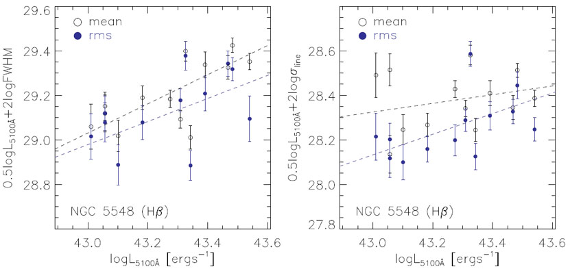Figure 6. A test on a non-zero using RM data for NGC 5548. Plotted here is the dependence of the virial products computed from 5100Å continuum luminosity and line width as a function of luminosity, for NGC 5548 and for H only, for FWHM (left) and line (right), respectively. This form of the virial product represents SE estimators with b = 0.5 and c = 2 in Eqn. (4), and I am using luminosity instead of time lag in computing the virial product since I am testing SE mass estimators. The measurements were taken from Collin et al. (2006), which are based on both mean and rms spectra during each monitoring period. Error bars represent measurement errors. The error bars in luminosity have been omitted in the plot for clarity. The continuum luminosity has been corrected for host starlight using the correction provided by Bentz et al. (2009a). The black and blue dashed lines are the best linear-regression fits using the Bayesian method of Kelly (2007), for measurements based on mean and rms spectra, respectively. The residual correlation between the virial product and luminosity cannot be completely removed, and a positive ~ 0.2 - 0.6 is inferred in all cases, although the uncertainty in is too large to rule out a zero at > 3 significance. Figure adapted from Shen & Kelly (2012).

A similar test is based on the repeated spectroscopy in SDSS (see discussion in Section 3.1.1). While most objects do not have a large dynamic range in luminosity variations in two epochs, the large number of objects allows a reasonable determination of the average trend of SE masses with luminosity, for the whole population of quasars. In addition, we want to include measurement uncertainties (both statistical and systematic), which allows us to make realistic constraints, as measurement errors will always be present. As shown in Fig. 1, the line width from single-epoch spectra does not seem to respond to luminosity variations except for low-luminosity objects based on H, as expected from the physical/practical reasons I described above. I plot the changes in SE masses as a function of luminosity changes in Fig. 7. From this figure I estimate ~ 0.5 for the high-L samples based on Mg II and C IV, and ~ 0 for the low-L sample based on H (She, Shen et al., in preparation). The difference in the low-L (low-z) and high-L (high-z) samples could be due to a luminosity effect, e.g., the correspondence between line width and luminosity variations is poorer at higher luminosities, or due to the difference between H and the other two lines (She, Shen et al., in preparation).

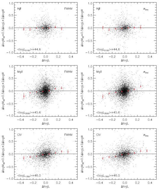Figure 7. Tests of a non-zero using two-epoch spectroscopy from SDSS (She, Shen, et al., in preparation). The data and notations are the same as in Fig. 1. The SE masses remain more or less constant as luminosity changes only for the low-luminosity and low-z sample based on H. For the high-luminosity and high-z samples based on Mg II and C IV, a luminosity-dependent bias in SE masses is inferred, with an error slope of ~ 0.5.

Shen & Kelly (2012) also attempted to constrain using forward Bayesian modeling of SDSS quasars in the mass-luminosity plane (see Section 4.2). While the results suggested a non-zero ~ 0.2-0.4, the constraints were not very strong (see their fig. 11). Combining all these tests, we can conclude the following: is probably smaller than ~ 0.5 (i.e., line width still plays some physical role in SE mass estimates) but unlikely zero, although the exact value is uncertain. The value of likely also depends on the specific line. More monitoring data of individual AGNs, and/or a substantially larger sample of AGNs with RM mass (or M_BH - _* masses) spreading enough dynamic range in luminosity at fixed mass, will be critical in better constraining .

The effects of the luminosity-dependent bias on flux-limited samples are discussed intensively in, e.g., Shen et al. (2008a), Shen & Kelly (2010) and Shen & Kelly (2012). Here I use a simple simulation of a power-law true BH mass distribution, dN / dM_BH M_BH^-3.6, to demonstrate these effects in Fig. 8. This steep true mass distribution was chosen to reproduce the distribution at the high-mass end for SDSS quasars (Shen et al. 2008a), which is certainly not appropriate at the low-mass end. I use the same example as in Fig. 5 for all the dispersion terms in luminosity and line width at fixed true mass. The true masses are distributed between 5 × 10⁷ M and 10¹⁰ M according to the specified power-law distribution. The mean luminosity at fixed m is determined assuming a constant Eddington ratio = 0.05. Then the instantaneous luminosity and SE mass at each true mass m are generated using Eqns. (13)-(19). The resulting distribution in the m-m_e plan is shown in black contours and points in Fig. 8, where I also show the distribution of a flux-limited (luminosity-limited) subset of BHs with l > <l>_m=8.3, the mean luminosity corresponding to M_BH = 2 × 10⁸ M. The simulated distributions in luminosity, line width and SE virial masses are consistent with those for SDSS quasars when a similar flux limit is imposed on the simulated BHs. It is clear from Fig. 8 that for the flux-limited subset, the SE masses are biased high from the true masses. This is because in this simulation we have = 0.49, which implies a significant luminosity-dependent bias at fixed true mass. Then the bottom-heavy BH mass distribution and the large scatter of luminosity at fixed true mass lead to more overestimated SE masses scattered upward than underestimated ones scattered downward, causing a net sample bias in SE masses (Shen et al. 2008a, Shen & Kelly 2010, Shen & Kelly 2012).

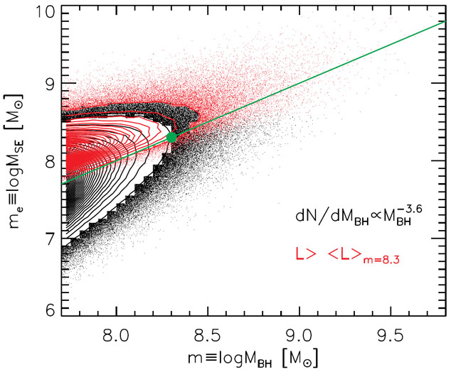Figure 8. A simulated population of BHs with true masses MBH within 5 × 107 - 1010 M, distributed as a power-law dN / dMBH MBH-3.6. I have assumed a constant Eddington ratio = 0.05 to generate the mean luminosity hlim at fixed true mass. I then used the dispersions specified by the example shown in Fig. 5 to generate instantaneous luminosity and SE masses. The resulting distributions in luminosity, line width and SE masses are consistent with those for the SDSS quasar sample (e.g., Shen et al. 2011). The black contours (local point density contours) and points show the distribution in the me - m plane. The green line shows the unity relation me = m. As expected, there is substantial scatter in me at fixed m due to the uncertainty in SE masses (SE = 0.42 dex). The red contours and points show the distribution for a subset of quasars with l > <l>m = 8.3, the corresponding mean luminosity at MBH = 2 × 108 M (marked by the green circle). The SE masses are biased high from their true masses for this flux-limited sample (i.e., most points are above the unity relation) due to the substantial luminosity-dependent bias, the large dispersion in luminosity at fixed true mass, and the bottom-heavy true mass distribution in this example

⁵ Some recent studies (e.g., Fine et al. 2011, Runnoe et al. 2013) argue that the dependence of line FWHM on source orientation is different for low-ionization and high-ionization lines, such that the C IV-emitting gas velocity field may be more isotropic than H and Mg II. Back.

⁶ Of some relevance here is the interpretation of the apparently small BH masses in a sub-class of Type 1 AGNs called narrow-line Seyfert 1s (NLS1s), where the H FWHM is narrower than 2000 km s^-1 along with other unusual properties (such as strong iron emission and weak [O III] emission). Some argue (e.g., Decarli et al. 2008b) that NLS1s are preferentially seen close to face-on, hence their virial BH masses based on FWHM are underestimations of true masses. However, NLS1s also differ from normal Type 1 objects in ways that are difficult to explain with orientation effects (such as weak [O III] and strong X-ray variability). Orientation may play some role in the interpretation of NLS1s (especially for a minority of radio-loud NLS1s), but is unlikely to be a major factor. Back.

⁷ Empirical iron emission templates in the rest-frame UV to optical can be found in, e.g., Boroson & Green (1992), Vestergaard & Wilkes (2001), Tsuzuki et al. (2006). Using different iron templates may lead to small systematic offsets ( 0.05 dex) in the measured continuum luminosity and line width (e.g., Nobuta et al. 2012). Occasionally a Balmer continuum component is added in the pseudo-continuum fit to improve the fit around the "small blue bump" region near 3000 Å (e.g., Grandi 1982, Dietrich et al. 2002), but such a component is generally difficult to constrain from spectra with limited wavelength coverage (see discussions in, e.g., Wang et al. 2009, Shen & Liu 2012). Back.

⁸ Here I give one possible derivation. For brevity I will drop m in all probability distributions, but it should be understood that all these distributions are at fixed m. Consider the '_w = 0 case first, where we want to derive p(m_e|l). Using Bayes's theorem, p(m_e|l) p(m_e)p(l|m_e). We have p(m_e) e^{-(m_e-m)2 / [2(b'_l)2]} (i.e., all variance in m_e comes from '_l since '_w = 0), and p(l|m_e) e^{-[l - (m_e-m / b + <l>_m)]2 / (2_corr2)} (i.e., l can only vary due to _corr at fixed m_e). Therefore p(m_e|l) e^{-(m_e - <m_e>_m,l)2 / (2_ml'2)}, where <m_e>_m,l is the same as in Eqn. (17), and _ml^'2 = (b'_l)² _corr² / (_l^'2 + _corr²). Now add back in the '_w term, which will convolve p(m_e|l) with a Gaussian distribution. Then the general distribution p(m_e|l) for arbitrary values of '_w is also a Gaussian, with the same mean, but a dispersion that is broadened by c'_w (i.e., the same as in Eqn. 17). Back.

⁹ For the sake of completeness, I note that > b could happen, if the line width were actually positively correlated to luminosity in the _corr terms in Eqn. (13). Of course such a scenario is counter-intuitive (regarding the virial assumption) and thus unlikely, and it means one should not use line width at all in estimating SE masses. Back.