4. APPLICATIONS TO STATISTICAL QUASAR SAMPLES

Despite the many caveats of SE mass estimators discussed above, they have been extensively used in recent years to measure BH masses in quasar and AGN samples over wide luminosity and redshift ranges, given their easiness to use. These applications include the Eddington ratio distributions of quasars, the demographics of quasars in terms of the black hole mass function (BHMF), the correlations between BH mass and host properties, and BH mass dependence of quasar properties. It is important to recognize, however, that these BH mass estimates are not true masses, and the uncertainty in these mass estimates has dramatic influences on the interpretation of these measurements.

Below I discuss several major applications of the SE virial mass estimators to statistical quasar samples. Other applications of these SE masses, such as quasar phenomenology, while equally important, will not be covered here.

4.1. Early Growth of SMBHs

One of the strong drivers for developing the SE virial mass technique is to estimate BH masses for high redshift quasars to better than a factor of ten accuracy, and to study the growth of SMBHs up to very high redshift (e.g., Vestergaard 2004). Such investigations have been greatly improved in the era of modern, large-scale spectroscopic surveys. The SDSS survey has been influential on this topic by providing more than tens of thousands of optical quasar spectra and SE mass estimates up to z ~ 5 (e.g., McLure & Dunlop 2004, Netzer & Trakhtenbrot 2007, Shen et al. 2008a, Shen et al. 2011, Labita et al. 2009a, Labita et al. 2009b). On the other hand, deeper and dedicated optical and near-IR spectroscopic programs are probing the SMBH growth to even higher redshift (e.g., Jiang et al. 2007, Kurk et al. 2007, Willott et al. 2010, Mortlock et al. 2011).

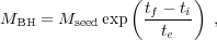
In Fig. 9 I show a compilation of SE virial mass estimates for quasars over a wide redshift range 0 < z 7 from different studies. The black dots show the SE masses from the SDSS DR7 quasar sample (Schneider et al. 2010, Shen et al. 2011), which were estimated based on H for z < 0.7, Mg II for 0.7 < z < 1.9 and C IV for 1.9 < z < 5. As discussed in Section 3.1.7, the reliability of C IV-based SE masses for the high-z and high-luminosity quasars has been questioned, and several studies have obtained near-IR spectra for z 2 quasars to get H-based (filled symbols) and Mg II-based (open symbols) SE masses at high redshift. Albeit with considerable uncertainties and possible biases in individual SE mass estimates (all on the order of a factor of a few), these studies show that massive, 10⁹ M BHs are probably already in place by z ~ 7, when the age of the Universe is only less than 1 Gyr. The abundance of these massive and active BHs then evolves strongly with redshift, showing the rise and fall of the bright quasar population with cosmic time.

Figure 9. A compilation of SE virial mass estimates from different samples of quasars. The black dots are the SE masses for SDSS quasars from Shen et al. (2011), based on H (z < 0.7), Mg II (0.7 < z < 1.9) and CIV (z > 1.9). Given the potential caveats of CIV-based SE masses, near-IR spectroscopy has been undertaken to estimate SE masses for z 2 quasars based on H and Mg II. The different large symbols are for SE masses based on H (filled symbols) and Mg II (open symbols) from Shemmer et al. (2004, filled squares), Netzer et al. (2007, filled circiles), Trakhtenbrot et al. (2011, open circles), Kurk et al. (2007, open triangles), Willott et al. (2010, open squares), and Mortlock et al. (2011, open circle with cross). Bear in mind the large uncertainty associated with individual SE masses and potential biases. I also show the predicted SMBH growth at z > 6 based on simple, continuous accretion models with constant Eddington ratio and radiative efficiency є = 0.1, as described in Eqn. (20). The solid lines are Eddington-limited ( = 1) growth models from a seed BH at z = 20; the dashed lines are = 1 growth models from a seed BH at z = 30; the dotted lines are mildly super-Eddington ( = 1.5) growth models from a z = 20 seed BH. For each model I used three seed BH masses, Mseed = 10, 20, 100 M to accommodate reasonable ranges of seed BH mass from a Pop III star remnant at z ~ 20 - 30.

One outstanding question regarding the observed earliest quasars is how they could have grown such massive SMBHs given the limited time they have, which is a non-trivial problem since the discoveries of z > 4 quasars (e.g., Turner 1991, Haiman & Loeb 2001). One concern is if these highest redshift quasars have their luminosities magnified by gravitational lensing or if their luminosities are strongly beamed (e.g., Wyithe & Loeb 2002, Haiman & Cen 2002), which will affect earlier estimates of their BH masses using the Eddington-limit argument. The lensing hypothesis will also lead to overestimated virial BH masses. However later deep, high-resolution imaging of z > 4 quasars with HST did not find any multiple images around these objects (e.g., Richards et al. 2004b, Richards et al. 2006b), rendering the lensing hypothesis highly unlikely (e.g., Keeton et al. 2005). Strong beaming can also be ruled out based on the high values of the observed line/continuum ratio of these high-redshift quasars (e.g., Haiman & Cen 2002).

Given the e-folding time introduced in Section 1, t_e = 4.5 × 10⁸ є / (1 - є) yr, and a seed BH mass M_seed at an earlier epoch z_i, the final mass at z_f ~ 6 is

(20)

where t_f and t_i are the cosmic age at z_f and z_i, respectively.

Assuming continuous accretion with constant radiative efficiency є and luminosity Eddington ratio and without mergers, I showed in Fig. 9 three different growth histories from a seed BH at higher redshift. The solid lines are for a seed BH at z = 20 and = 1, i.e., Eddington-limited accretion; the dashed lines are for a seed BH at z = 30 and = 1; the dotted lines are for a seed BH at z = 20 and = 1.5, i.e., mildly super-Eddington accretion. For each model I used three seed BH mass, M_seed = 10,20,100 M, which encloses the reasonable ranges of predicted remnant BH mass from the first generation of stars (Pop III stars, for a review see, e.g., Bromm et al. 2009). Then it is clear from Fig. 9 that, if the accretion is Eddington-limited, it is difficult to grow 10⁹ M BHs at z ~ 6 from a Pop III remnant seed BH at z ~ 20-30 (where such first stars were formed out of ~ 10⁶ M halos, corresponding to ~ 3-4 peaks in the density perturbation field). On the other hand, if allowing mildly super-Eddington accretion, then a ~ 10⁹ M BH can be readily formed at z ~ 7 from a large Pop III star remnant M_seed ~ 100 M, although more recent simulations suggest somewhat lower masses of Pop III stars due to possible effects of clump fragmentation and/or radiative feedback (e.g., Turk et al. 2009, Hosokawa et al. 2011, Stacy et al. 2012), and hence a lower typical value of the remnant mass of less than tens of solar masses. Mildly super-Eddington accretion (up to ~ a few) could happen, for instance, if the radiation and density fields of the accretion flow are anisotropic and most of the accretion flow is not impeded by the radiation force. Mergers between BHs at high-z can also help with the required growth if the coalesced BH is not ejected from the halo by the gravitational recoil from the merger. The main challenge here is whether or not such critical accretion can maintain stable and uninterrupted for the entire time (e.g., Pelupessy et al. 2007). But in any case, it is quite likely that the observed z > 6 quasars are all born in rare environments of the early Universe, thus extreme conditions (such as large gas density, high merger rate, etc.) may have facilitated their growth. Indeed, some theoretical studies can successfully produce such massive BHs at z ~ 6 growing from a typical Pop III remnant BH seed without super-Eddington accretion (e.g., Yoo & Miralda-Escude 2004, Li et al. 2007, Tanaka & Haiman 2009). But the detailed physics (accretion rate, mergers, BH recoils, etc.) regarding the formation of these earliest SMBHs is still uncertain to some large extent.

While this is not seen as an immediate crisis, there are multiple pathways to make it much easier to grow 10⁹ M SMBHs at z 6 by boosting either the accretion rate or the seed BH mass (for a recent review, see, e.g., Volonteri 2010, Haiman 2012). These recipes include:

1) supercritical accretion (e.g., Volonteri & Rees 2005) where the accretion rate _BH greatly exceeds the Eddington limit with a canonical radiative efficiency є = 0.1. One possibility is that the radiation is trapped in the accretion flow (e.g., Begelman 1979, Wyithe & Loeb 2012), leading to a very low є and hence a much shorter e-folding time. Note that in such a radiatively inefficient accretion flow (RIAF), the luminosity is still bounded by the Eddington limit;

2) rapid formation of massive (~ 10³-10⁵ M) BH seeds from direct collapse of primordial gas clouds (e.g., Bromm & Loeb 2003, Begelman et al. 2006, Agarwal et al. 2012) or from a hypothetical supermassive star or "quasi-star" (e.g., Shibata & Shapiro 2002, Begelman et al. 2008, Johnson et al. 2012) at high redshift. Supercritical accretion may also be expected in some of these models to grow to the final seed BH mass, which then continue to accrete in the normal way. By increasing M_seed it requires much less e-folds to grow to a > 10⁹ M BH. Another possible route to produce massive BH seeds up to ~ 10³ M is by the runaway collisional growth in a dense star cluster formed in a high-redshift halo (e.g., Omukai et al. 2008).

4.2. Quasar Demographics in the Mass-Luminosity Plane

BH mass estimates provide an additional dimension in the physical properties of quasars. The distribution of quasars in the two-dimensional BH mass-luminosity (M - L) plane conveys important information about the accretion process of these active SMBHs. The first quasar mass-luminosity plane plot was made by Dibai in the 1970s as mentioned in Section 2.2. Over the years, such a 2D plot has been repeatedly generated based on increasingly larger quasar samples and improved BH mass estimates (e.g., Wandel et al. 1999, Woo & Urry 2002, Kollmeier et al. 2006, Shen et al. 2008a, Shen & Kelly 2012), and the much better statistics now allows a more detailed and deeper look into this quasar mass-luminosity plane.

In what follows I will mainly focus on the SDSS quasar sample because this is the largest and most homogeneous quasar samples to date. But as emphasized in Shen & Kelly (2012), the SDSS sample only probes the bright-end of the quasar population, and to probe the mass and accretion rate of the bulk of quasars it is necessary to assemble deeper spectroscopic quasar samples (e.g., Kollmeier et al. 2006, Gavignaud et al. 2008, Trump et al. 2009, Nobuta et al. 2012).

Since I have emphasized the distinction between true BH masses and SE mass estimates, I shall use the term "observed" or "measured" to refer to distributions based on SE mass estimates, to distinguish them from "true" distributions. Fig. 10 shows such an observed mass-luminosity plane from the same collection of quasars as shown in Fig. 9. Note that these samples are flux-limited to different magnitudes, and several high-redshift samples based on H or Mg II (i.e., large symbols) have a higher flux-limit than the SDSS. I also used slightly different values of bolometric corrections to convert continuum luminosity to bolometric luminosity for those non-SDSS samples. From this plot we see that the observed distributions of quasars are bounded between constant Eddington ratios 0.01 1, with median values of < > ~ 0.1-0.3 for SDSS quasars, and somewhat higher values for the z 5 samples. The dispersion in Eddington ratio in these flux-limited samples is typically ~ 0.3 dex. Similar distributions were observed by, e.g., Kollmeier et al. (2006). However, as demonstrated in, e.g., Shen et al. (2008a), Kelly et al. (2009a, 2010), Shen & Kelly (2012), Kelly & Shen (2013), the observed distribution suffers from the sample flux limit such that low-Eddginton ratio objects have a lower probability being selected into the sample, and from the uncertainties and statistical biases of SE masses relative to true masses. The selection effect due to the flux limit and errors in SE masses dramatically modify the intrinsic distribution in the mass-luminosity plane, and must be taken into account when interpreting the observations.

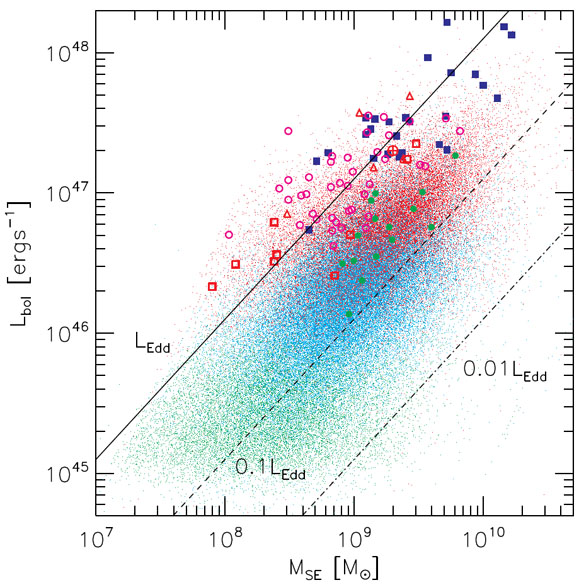Figure 10. The observed quasar mass-luminosity plane based on SE masses for quasars in a wide range of redshifts (0 < z 7) from the samples compiled in Fig. 9. The dots are from the SDSS sample in Shen et al. (2011), for quasars at z < 0.7 (H-based SE masses; green), 0.7 < z < 1.9 (Mg II-based SE masses; cyan), and 1.9 < z < 5 (CIV-based SE masses; red). The large symbols are from various z 2 samples using H or Mg II-based SE masses. I have used slightly different bolometric corrections for these non-SDSS samples from those used in the original papers. The SDSS quasars have Eddington ratios 0.01 1 with a mean value of <> ~ 0.1 - 0.3, while the other high-z samples have even higher Eddington ratios. Given the fluxlimited nature of all these samples and the errors in SE masses, the observed Eddington ratio distribution is highly biased relative to the intrinsic distribution (see Section 4.2 for details).

The best approach to tackle these issues is a forward modeling, in which one specifies an underlying distribution of true masses and luminosities and map to the observed mass-luminosity plane by imposing the flux limit and relations between SE virial masses and true masses (e.g., Shen et al. 2008a, Kelly et al. 2009a, Kelly et al. 2010). Then the comparisons between model and observed distributions constrain the model parameters with standard Markov Chain Monte Carlo (MCMC) techniques and Bayesian inference. This is a complicated and model-dependent problem, and the best efforts so far are the studies by Shen & Kelly (2012) and Kelly & Shen (2013), building on earlier work by Shen et al. (2008a), Kelly et al. (2009a) and Kelly et al. (2010). Alternatively, Schulze & Wisotzki (2010) developed a maximum likelihood method (also a forward modeling method), which accounts for the effect of the flux limit, but not the errors in SE masses (although the SE errors can be incorporated in such a framework as well). This maximum likelihood method was subsequently adopted in Nobuta et al. (2012) when modeling a faint quasar sample (again, SE errors not taken into account). Most other quasar mass demographic studies, however, did not explicitly model either of these effects (e.g., Greene & Ho 2007, Vestergaard et al. 2008, Vestergaard & Osmer 2009).

Shen & Kelly (2012) used forward modeling with Bayesian inference to model the observed distribution in the mass-luminosity plane of SDSS quasars, taking into account a possible luminosity-dependent bias (i.e., ≠ 0, see Section 3.3.2) to be constrained by the data. The flux limit of the SDSS sample is taken into account using published selection functions of SDSS quasars (Richards et al. 2006a). Based on this approach, Shen & Kelly (2012) found evidence for a non-zero , although the constraints on are weak and cannot rule out a null value. Kelly & Shen (2013) used a more flexible model parametrization to describe the underlying true distributions (in BH mass and Eddington ratio), but fixed = 0 to test how sensitively the results in Shen & Kelly (2012) depend on different model parameterizations. They found that the main conclusions are generally consistent, although the results in the latter work are less constrained than in the former, due to the more flexible models. Both studies revealed that based on the SDSS quasar sample alone, it is difficult to constrain the BHMF to better than a factor of a few at most redshifts. This is both because the SDSS sample only probes the tip of the active SMBH population at high-z, and to a larger extent, because the errors of SE masses are poorly understood. However, there are some solid conclusions from the two studies:

1. The observed distribution in the mass-luminosity plane is quite different from the intrinsic distribution, due to the flux limit and uncertainties in SE masses. This is demonstrated in Fig. 11, which shows a quasar M - L plane at z = 0.6 based on the modeling of SDSS quasars by Shen & Kelly (2012). In this plot luminosity L is the restframe 2500 Å monochromatic luminosity, and the bolometric luminosity is L_bol ~ 5L. The red contours are the true distribution of quasars, while the black contours are the measured distribution based on H SE virial masses. The black horizontal line indicates the flux limit of the sample, hence only objects above this line would be selected in the SDSS sample, which form the observed distribution. The flux limit only selects the most luminous objects into the SDSS sample, missing the bulk of low Eddington ratio objects; even the highest mass bins are incomplete due to the flux limit. The distribution based on SE virial BH masses is flatter than the one based on true masses due to the scatter and luminosity-dependent bias of these SE masses.

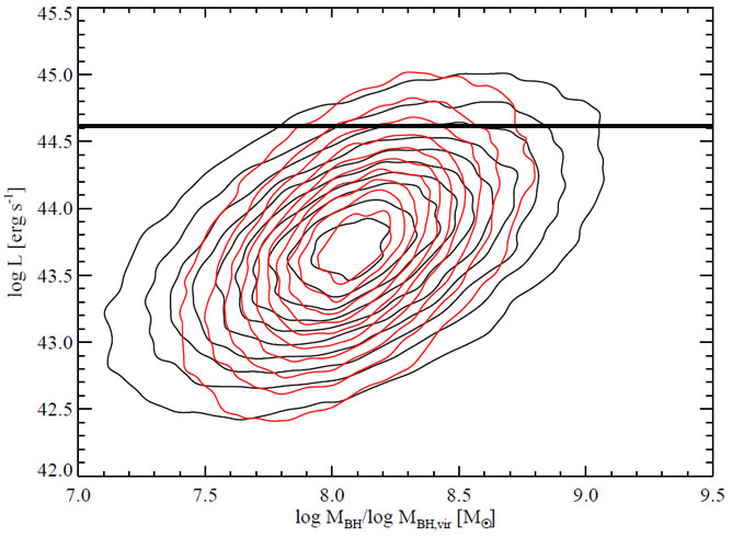   Figure 11. The simulated mass-luminosity plane at z = 0.6 based on the modeling of SDSS quasars in Shen & Kelly (2012), which extends below the flux limit (the black horizontal line). The y-axis plots the restframe 2500Å monochromatic luminosity, and the bolometric luminosity is Lbol ~ 5L. The red contour is the distribution based on true BH masses and is determined by the model BHMF and Eddington ratio distribution in Shen & Kelly (2012). The black contour is the distribution based on H SE BH masses. The flux limit only selects the most luminous objects into the SDSS sample (which are closer to the Eddington limit), and the distribution based on SE virial BH masses is flatter than the one based on true masses due to both the scatter ml and a non-zero ~ 0.2 for this redshift bin (see Section 3.3.2 and Shen & Kelly 2012).

   For the observed distribution based on SE masses, there are fewer objects towards larger SE masses and luminosity. This was interpreted as the lack of massive black holes accreting at high Eddington ratios, or the so-called "sub-Eddington boundary" claimed by Steinhardt & Elvis 2010a. However, such a feature is caused by the flux limit and errors in SE masses, and there is no evidence that high-mass quasars on average accrete at lower Eddington ratios, not for broad-line objects at least ¹⁰. This conclusion seems to be robust against different model parameterizations of the underlying true distributions in the forward modeling approach (Kelly & Shen 2013). Of course here I am assuming no systematic biases in these FWHM-based SE masses measured in Shen et al. 2011. It is possible that _line-based SE masses are more reliable, in which case there would be a "rotation" in the mass-luminosity plane using _line-based SE masses, as discussed in Section 3.1.3. This also tends to reduce this "sub-Eddington boundary" in the observed plane (e.g., Rafiee & Hall 2011a, Rafiee & Hall 2011b), but a full modeling taking into account both the flux limit and SE mass errors is yet to be performed with _line-based SE masses (i.e., the interpretation by Rafiee & Hall is still based on "observed" rather than true distributions).

2. The intrinsic Eddington ratio distribution at fixed true mass is broader (~ 0.4 dex) than the observed Eddington ratio distribution in flux-limited samples ( 0.3 dex), and the mean Eddington ratio in the flux-limited samples based on SE masses is higher ¹¹ than the mean Eddington ratio for all active SMBHs (most of which are not detected). This is consistent with earlier studies by Shen et al. (2008a) and Kelly et al. (2010). Some deeper spectroscopic surveys indeed start to find these lower Eddington ratio objects (e.g., Babic et al. 2007, Gavignaud et al. 2008, Nobuta et al. 2012), and are consistent with the model-extrapolated distributions from Shen & Kelly (2012) and Kelly & Shen (2013); however, since in general these deep data are noisier and the selection function is less well quantified than SDSS, care must be paid when inferring the dispersion in Eddington ratios for these faint quasars.

The next step to utilize this quasar mass-luminosity plane is to measure the abundance of quasars in this plane, and study its redshift evolution. This is a much more powerful way to study the cosmic evolution of quasars than traditional 1D distribution functions such as the luminosity function (LF) and the quasar BHMF.

I demonstrate the power of the mass-luminosity plane in quasar demographic studies in Fig. 12. This is the same simulated, true quasar M - L plane at z = 0.6 as in Fig. 11, using the models in Shen & Kelly (2012) constrained using SDSS quasars. The 2D density (i.e., abundance) of quasars in this plane is shown in the color-coded contours. The traditional LF and BHMF (shown in the right panels) are then just the projection onto each axis. In the right panels I also demonstrate the differences between using true BH masses and SE virial masses, as well as the effect of the sample flux limit. It is clear from this demonstration that the 1D distribution functions lose information by collapsing on one dimension, and a better way to study the demography of quasars is to measure their abundance in 2D, since the mass and luminosity of a quasar are physically connected by the Eddington ratio. The ultimate goal is to study the evolution of the quasar density in the M - L plane as a function of time. Recent studies have started to work in this direction (e.g., Shen & Kelly 2012, Kelly & Shen 2013), although deeper quasar samples and a better understanding of SE mass errors are needed to utilize the full power of the M - L plane.

Figure 12. An example of the forward modeling of quasar demographics in the mass-luminosity plane by Shen & Kelly (2012), modeled at z = 0.6. Left: The simulated mass-luminosity plane (with true BH masses), which extends below the SDSS flux limit (the black horizontal line). Shown here is the comoving number density map [(MBH, L)], where only regions with (MBH, L) > 10-6.5 Mpc-3 log L-1 log MBH-1 are shown. The two diagonal lines indicate constant Eddington ratios of 1 and 0.01. The flux limit only selects the most luminous objects into the SDSS sample. Right: Projections of the 2D distribution onto the luminosity and BH mass axes, i.e., the LF (upper right) and BHMF (bottom right) of quasars at z = 0.6. The points are binned observational data and the lines are best-fit models: the magenta lines show the results for all broad-line quasars (corrected for the flux limit) and the green lines show those for the flux-limited sample. The thickness of the lines indicates the 1 model uncertainty. I have used the i-band absolute magnitude instead of bolometric luminosity in presenting the LF, and I have also taken into account the difference between true BH masses (colored lines) and SE virial BH masses (points). This forward-modeling framework accounts for the selection incompleteness in BH mass due to the flux limit, and the uncertainties in SE virial BH mass estimates, and can constrain the 2D distribution down to ~ 3 magnitudes fainter than the flux limit (Shen amp; Kelly 2012). However, to make more robust constraints at the faint end, deeper quasar samples are highly desirable.

To summarize, the quasar mass-luminosity plane has great potential in studying quasar evolution, and efforts have been underway to investigate this plane in detail (e.g., Steinhardt & Elvis 2010a, b, Steinhardt et al.2011, Steinhardt & Elvis 2011, Shen & Kelly 2012, Kelly & Shen 2013). However, it should always be kept in mind that the "observed" distribution in the M - L plane is not the true distribution. I strongly discourage direct interpretations of the observed distributions based on SE masses and flux-limited data, which can easily lead to superficial or even spurious results.

4.3. Evolution of BH-Bulge Scaling Relations

Another important application of SE virial mass estimators is to study the M_BH-host scaling relations in broad line AGNs, and to probe the evolution of these relations at high redshift. Measuring the M_BH-host relations in low redshift quasars and AGNs has been done using both RM masses and SE masses (e.g., Laor 1998, Greene & Ho 2006, Bentz et al. 2009c, Xiao et al. 2011). Assuming some virial coefficient < f >, these studies were able to add active objects in these scaling relations and extend the dynamic range in BH mass.

In the past a few years, there have been a huge amount of effort to quantify the evolution of these scaling relations up to z ~ 6, by measuring host properties in broad-line quasars. Some studies directly measure the galaxy properties by decomposing the quasar and galaxy light in either imaging or spectroscopic data (e.g., Treu et al. 2004, Peng et al. 2006a, b, Woo et al. 2006, Treu et al. 2007, Woo et al. 2008, Shen et al. 2008b, Jahnke et al. 2009, McLeod & Bechtold 2009, Decarli et al. 2010, Merloni et al. 2010, Bennert et al. 2010, Cisternas et al. 2011, Targett et al. 2012); other studies use indirect methods to infer galaxy properties, such as using the narrow emission line width to infer bulge velocity dispersion (e.g., Shields et al. 2003, 2006, Salviander et al. 2007, Salviander & Shields 2012). Molecular gas (using CO tracers) has also been detected in the hosts of z ~ 6 quasars, allowing rough estimates on the host dynamical mass of these highest redshift quasars (e.g., Walter et al. 2004, Wang et al. 2010 and references therein). In all cases the BH masses were estimated using the SE methods based on different broad emission lines. With a few exceptions, most of these studies claim an excess in BH mass relative to bulge properties either in the M_BH - _* relation or in the M_BH - M_bulge / L_bulge relation, and advocate a scenario where BH growth precedes spheroid assembly.

It is worth noting that measuring host galaxy properties of Type 1 AGNs could be challenging, and systematic biases may arise when measuring the stellar velocity dispersion from spectra (e.g., Bennert et al. 2011), or host luminosities from image decomposing (e.g., Kim et al. 2008, Simmons & Urry 2008). Conversions from measurables (such as host luminosity) to derived quantities (such as stellar mass) are also likely subject to systematics, especially for low-quality data. Thus careful treatments are required to derive unbiased host measurements.

On the other hand, it is also worrisome that the errors in SE BH mass estimates may affect the observed offset in the BH scaling relations at high-redshift. As discussed extensively in Section 3, there are both physical and practical concerns that the applications of locally-calibrated SE estimators to high-redshift quasars may cause systematic biases. Even if the extrapolations are valid, the luminosity-dependent bias discussed in Section 3.3.2 may still lead to an average overestimation of quasar BH masses in flux-limited surveys. (Shen & Kelly 2010) studied the impact of the luminosity-dependent bias on flux-limited quasar samples, and found an "observed" BH mass excess of ~ 0.2-0.3 dex for L_bol 10⁴⁶ erg s^-1 with a reasonable value of '_l = 0.4 dex (see Section 3.3.2 for details). This sample bias using SE mass estimates becomes larger (smaller) at higher (lower) threshold quasar luminosities.

Another statistical bias was pointed out by Lauer et al. (2007), which is at work even if there is no error in BH mass estimates. The basic idea is that since there is an intrinsic scatter between BH mass and bulge properties (~ 0.3 dex for the local sample), and since the distribution functions in BH mass and galaxy properties are expected to be bottom-heavy, a statistical excess (bias) in the average BH mass relative to bulge properties arises when the sample is selected based on BH mass (or based on quasar luminosity, assuming the Eddington ratio is constant). This is similar to the Malmquist-type bias discussed in Section 3.3.1. One can work out (e.g., Lauer et al. 2007, Shen & Kelly 2010) that the BH mass offset introduced by this bias depends on the slope of the galaxy distribution function, as well as the scatter in the BH-host scaling relations. For simple power-law models of the galaxy distribution function on property S with a slope _s, and lognormal scatter _µ at fixed galaxy property S, this bias takes a similar form as the Malmquist-type bias in Section 3.3.1:

(21)

where C is the coefficient of the mean BH-host property (S) scaling relation logM_BH = C logS + C'. Thus if the intrinsic scatter in the BH-host scaling relations increases with redshift, then this statistical bias alone can contribute a significant amount to the observed BH mass offset in the high-redshift samples (e.g., Merloni et al. 2010). A larger intrinsic scatter in these scaling relations at high redshift is expected, if the tightness of the local BH-host scaling relations is mainly established via the hierarchical merging of less-correlated BH-host systems at higher redshift (e.g., Peng 2007, Hirschmann et al. 2010, Jahnke & Macció 2011). The real situation is of course more complicated, and one must consider a realistic Eddington ratio distribution at fixed BH mass and the effect of the flux limit. There could also be other factors that may complicate the usage of AGNs to probe the evolution of these BH-host scaling relations, as discussed in detail in Schulze & Wisotzki (2011). But overall a BH mass excess due to the Lauer et al. bias is expected when select on quasar luminosity. An interesting corollary is that a deficit in BH mass is expected if the sample is selected based on galaxy properties. This may explain the findings that high-redshift submillimeter galaxies (SMGs) tend to have on average smaller BHs relative to expectations from local BH-host scaling relations (e.g., Alexander et al. 2008).

The Lauer et al. bias caused by the intrinsic scatter in BH-host scaling relations works independently with the luminosity-dependent bias caused by errors in SE masses, so together they can contribute a substantial (or even full) amount of the observed BH mass excess at high redshift (e.g., Shen & Kelly 2010). Both biases are generally worse for samples with a higher luminosity threshold given the curvature in the underlying distribution function ¹², thus higher-z samples with higher intrinsic AGN luminosities will have larger BH mass biases, leading to an apparent evolution. There are several samples that are probing similar luminosities as the local RM AGN sample (e.g., Woo et al. 2006). Since the SE mass estimators were calibrated on the local M_BH - _* relation using the RM AGN sample, one argument often made is that both biases should be calibrated away for the high-z sample with similar AGN luminosities. This argument is flawed, however, because the local RM AGN sample is heterogeneous and is not sampling uniformly from the underlying BH/galaxy distribution functions, while the high-z sample usually is sampling uniformly from the underlying distributions – this is exactly why both biases will arise for the high-z samples. The only exception that might work is to compare two quasar samples at two different redshifts with the same luminosity threshold, where the predicted BH mass biases should be of the same amount, and see if there is evolution in the average host properties. But even in this case it requires that the underlying distributions (slope and scatter) and measurement systematics are the same for both the low-z and high-z samples. Proper simulations that take into account the measurement systematics (in both BH mass and host properties) and underlying distributions should be performed to verify the interpretations upon the observations.

To summarize, there might be true evolutions in the BH-host scaling relations ¹³, but the current observations are inconclusive, due to the unknown systematics in the BH mass and host galaxy measurements. Better understandings of these systematics, the selection effects, as well as theoretical priors are all needed to probe the evolution of these scaling relations, and such efforts have been underway (e.g., Croton 2006, Robertson et al. 2006, Lauer et al. 2007, Hopkins et al. 2007, Di Matteo et al. 2008, Booth & Schaye 2009, Shankar et al. 2009, Shen & Kelly 2010, Hirschmann et al. 2010, Schulze & Wisotzki 2011, Jahnke & Macció 2011, Portinari et al. 2012, Salviander & Shields 2012, Zhang et al. 2012).

¹⁰ There could be a significant population of high-mass, non-broad-line AGNs accreting at low Eddington ratios, possibly via a different accretion mode than broad line quasars. Back.

¹¹ These SE masses are on average overestimated due to the luminosity-dependent bias discussed in Section 3.3.2, which tends to underestimated the true Eddington ratios. But the mean observed Eddington ratio based on SE masses of the flux-limited sample is still higher than the mean value for all quasars extending below the flux limit (see fig. 19 of Shen & Kelly 2012). Back.

¹² This is not always the case. If the scatter (_µ, '_l) increases at the low-mass end, then both biases could be worse at the low-mass/luminosity end. Back.

¹³ If the mass and velocity dispersion of galaxies bear any resemblance to the virial mass (M_{h, vir}) and virial velocity (V_h,vir) of their host dark matter halos, then one of the two relations, M_BH - _* and M_BH - M_bulge, must evolve since the M_h,vir - V_h,vir relation is redshift-dependent. Back.