


The process that governs galaxy formation is the collapse of gravitationally unstable regions, and in some aspects resembles the process of star formation discussed above. The most likely origin of the initial perturbations is inflation, an epoch of exponential expansion of the Universe, during which quantum fluctuations in the field driving the inflation (the inflaton) were stretched to macroscopic scales. The exact nature of the inflaton is not yet known, but the basic predictions of the theory are confirmed by observations, in particular the flatness of the Universe [30].
There are three types of metric perturbations: scalar, vector and tensor. Vector and tensor perturbations decay (in the matter-dominated era) in an expanding Universe, and the large-scale structure is seeded by the scalar perturbations, since these are coupled to the stress-energy tensor of the matter-radiation field.
Scalar perturbations can be classified into perturbations of the spatial curvature (commonly referred to as adiabatic) and perturbations in the entropy. Adiabatic perturbations arise if the relative number densities of all species remain constant: δ(nγ / nb) = 0, δ(nγ / nm) = 0 and so on. In this case there is no energy transfer between the various components, the energy conservation equation is satisfied by each component separately and we obtain the familiar results: ρm a3 = const., ρb a3 = const. and ργa4 = const. Therefore:
 |
(12) |
Entropy perturbations can be defined as deviations from adiabaticity, for example for dark matter and radiation:
 |
(13) |
and similarly for other pairs of species.
These two types of fluctuations are orthogonal, in the sense that all other types can be described as a linear combination of adiabatic and entropy modes which evolve independently.
The most natural, single-field inflationary models typically produce adiabatic fluctuations, and these predictions agree well with observations [31]. However, a sub-dominant isocurvature component might exist and lead to observable effects, such as blue tilted scale-dependent spectra or to non-gaussian density perturbations [32].
These initial conditions were set by the end of the inflationary period, when the Universe was ~ 10-35 second old. The primordial curvature perturbations were then at a level of ~ 10-5 and provided the seeds for future formation of structure in the universe.
In order to understand the evolution of the density fluctuations in the expanding Universe we need to solve the perturbed Friedmann equations. However, when the scale of the perturbation is small compared to the horizon (ℓ ≪ ct0) and the flow is non-relativistic (v ≪ c), a Newtonian derivation can be used. Furthermore, when the perturbations are still small, as happens in the early stages of structure formation, the equations that govern their evolution can be linearized.
We begin with the equation of mass conservation:
 |
(14) |
the Euler equation:
 |
(15) |
the Poisson equation:
 |
(16) |
and an equation of state: P = P(ρ). If the flow is homogeneous, the solution to the above equations is:
 |
(17) |
Now we perturb this solution as follows:
 |
(18) |
and define the comoving coordinate x = r / a(t) and the proper time dτ = dt / a. We obtain the following equations, where all the time and spatial derivatives are with respect to τ and x:
 |
(19) |
 |
(20) |
and
 |
(21) |
If the perturbations are small, we can linearize the equations, so that the
first equation becomes
 + ∇ ⋅
v = 0 and solve for δ.
Note that from the condition of adiabaticity (no heat exchange between fluid
elements) it follows that:
+ ∇ ⋅
v = 0 and solve for δ.
Note that from the condition of adiabaticity (no heat exchange between fluid
elements) it follows that:
 |
(22) |
where cs = √dP / dρ is the speed of sound and the last equality is the result of linearization.
The velocity field can be decomposed as follows:
 = || +
⊥
where
= || +
⊥
where
 ×
|| = 0 and
⋅
⊥ = 0.
The rotational component, equivalent to a vorticity, satisfies:
×
|| = 0 and
⋅
⊥ = 0.
The rotational component, equivalent to a vorticity, satisfies:
 |
(23) |
and therefore decays in the expanding Universe. The irrotational component satisfies:
 |
(24) |
Peculiar velocities associated with this component arise due to density fluctuations.
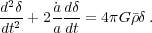
Finally, combining eqs. (19)-(21) and moving back to physical units, we obtain the following equation for the overdensity field:
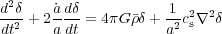 |
(25) |
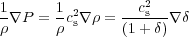
where the second term on the left is the damping term due to the expansion of the Universe, the first term on the right is the gravitational driving term and the second term on the right represents the pressure support.
Now let us decompose δ into plain wave modes δ(x, t) = Σ δk eix ⋅ k where λ = 2π a / k is the physical wavelength. The perturbation is unstable if its scale exceeds the Jeans scale, defined here as:
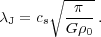 |
(26) |
In the case of weakly interacting dark matter the matter pressure vanishes and eq. (25) reduces to:
 |
(27) |
During the epoch of matter domination, ρm > ργ and all the wavelengths are unstable. A lower bound arises due to the free streaming of the dark matter particles, and corresponds to the cosmologically irrelevant scale of ~ 10-6 Earth mass for a 100 GeV dark matter particle. In fact there are interesting variations in this scale that arise from considerations of kinetic as opposed to thermal decoupling [33] and from the possible dominance of warm dark matter [34].
In an Einstein-de Sitter background (Ωm = 1), the scale factor grows as a ∝ t2/3 while ρ = ρm ∝ a-3 and there are two solutions to eq. (27): δ∝ t2/3 and δ∝ t-1. At late epochs, the constant energy density associated with the cosmological constant dominates over matter and the solution is δ ≈ const.
Recall that in the general case the background Universe is governed by the following equation:
 |
(28) |
One solution to the perturbation equations is therefore:
 |
(29) |
In other words, the overdensity is nearly constant during radiation domination (in fact it grows logarithmically), and grows as t2/3 in the matter domination epoch.
These results can be reformulated statistically by Fourier transforming these equations and looking at the power spectrum of the density fluctuations:
 |
(30) |
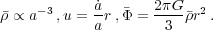
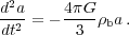
where P(k) = Akn. For large scales, n ≃ 1 (for example, from measurements of the cosmic microwave background anisotropies [30]) while on small scales, growth is suppressed during radiation domination, which results in a characteristic peak in P(k) on a scale corresponding to matter-radiation equality. From eq. (30) it follows that δ ρ / ρ ∝ k(n+3)/2 or δρ / ρ ∝ M-(n+3)/6. Asymptotically for large M, δρ / ρ ∝ M-2/3. More precisely, the power spectrum today can be described by Pobs(k) ∝ kn T2(k) where T(k) is a transfer function which represents the modifications to the primordial power spectrum due to the transition from radiation to matter domination. The power spectrum observed on different scales is shown schematically in fig. 7. This figure nicely illustrates the complementarity of diverse observations that either directly (CMB) or indirectly (clusters, galaxies, IGM) sample the linear density fluctuation spectrum.
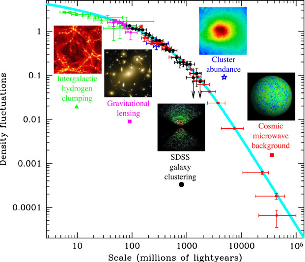 |
Figure 7. Power spectrum measurements (dots) and the theoretical prediction (blue curve). Image credit: M. Tegmark (SDSS). |
When the fluctuations are large enough so that δ ≃ 1, the linear approximation breaks down and a full solution for the non-linear equations is needed. In the general case, eqs. (14)-(16) cannot be solved analytically and it is necessary to use numerical simulations to obtain the matter distribution at late times.
The general scheme for structure formation in a cold-dark matter dominated universe was proposed in [35]. Dissipation was incorporated and a two-stage theory of baryonic cores in CDM halos was first described by [36]. We develop these arguments below via describing the recent simulations but first give the only analytical results for fully nonlinear dissipationless dark matter structures.
An exact solution exists for the nonlinear evolution of a spherically symmetric density perturbation [37] (a pedagogical treatment is given in [38]). Consider a mass M enclosed in a spherical volume with radius R and constant overdensity relative to the background universe 1 + δ = 3M / 4π R3 ρb, where ρb is the background density. By Birkhoff's theorem, the evolution of this spherical region is determined solely by its mass:
 |
(31) |
while the expansion of the background universe in the Einstein-de Sitter case is given by:
 |
(32) |
Thus, the overdense spherical region evolves like a Universe with a different mean density but the same initial expansion rate. Integration of eq. (31) gives:
 |
(33) |
where E is the energy of the spherical region. In analogy with
the background Universe, if E < 0 the overdense region behaves
like a closed universe and collapses, whereas for E > 0,
 is always positive
and the spherical region continues to expand forever.
is always positive
and the spherical region continues to expand forever.
The solution to eq. (33) is given in parametric form by:
 |
(34) |
and
 |
(35) |
where the constants A and B are related by A3 = GMB2. The parameter θ increases with t, while R increases to a maximum value Rm = 2A called the turnaround radius at θ = π and t = π B and then decreases to zero at tcoll = 2tm.
However, in reality the spherical perturbation does not collapse to a point but, at least in the case of dissipationless collapse, attains a finite radius, taken here to be the virial radius at which the kinetic and gravitational energies satisfy |U| = 2K. At the turnaround radius the kinetic energy vanishes, and the total energy is E = U = -3GM2 / 5Rm. At virialization, the total energy is E = U + K = U/2 = -3GM2 / 10Rvir. Equating the last two expressions we conclude that the virialization radius satisfies Rvir = Rm / 2. Consequently, the nonlinear overdensity at virialization ΔV ≡ 1 + δ is not infinite.
In order to relate to the linear theory developed above, we expand eqs. (34)-(35) in powers of small θ and then eliminate θ:
 |
(36) |
For t → 0, we recover the background scale factor:
 |
(37) |
which, as expected, evolves like Rb ∝ t2/3. The linear overdensity is given by 1 + δ = Rb3 / Rlin3 which, after using the above expressions and expanding to lowest order in t results in:
 |
(38) |
Consequently, the linear overdensity at the time of collapse t = tcoll is δc = (12π)2/3 3/20 = 1.686. This result should be understood in the following way: clearly the linear approximation breaks down long before the spherical region collapses, however if we continue to evolve the linear overdensity field as a mere mathematical construct, it would have obtained the value δc when the real spherical overdensity collapses.
In order to find the true overdensity at virialization, we first calculate the overdensity at the turnaround point: 1 + δ = Rb3(tm) / Rm3 = 9π2 / 16. As we have seen, the radius at virialization is reduced by a factor of 2, therefore the density increases by a factor of 8, while the background density decreases by a factor of Rb3(tcoll) / Rb3(tm) = (tcoll / tm)2 = 4. Thus, the overdensity at virialization is given by:
 |
(39) |
Another, almost exact, solution exists for one-dimensional collapse and is a variant of the Zeldovich approximation [39]. Imagine a homogeneous medium perturbed by a sinusoidal wave of wavelength Ld, such that the positions are given by:
 |
(40) |
where Zi are the initial positions, a(t) is the growth factor and ap defines the amplitude of the perturbation. Using the mass conservation equation for the one-dimensional case we obtain the density distribution:
 |
(41) |
In this case, a caustic singularity develops for Zi = nLd / 2. This simplified analysis demonstrates the formation of caustics, which is also seen as sheets and filaments in numerical simulations of the so-called cosmic web of large-scale structure [40].
The spherical collapse model discussed above is the basis for the calculation of the halo mass function, or the abundance of virialized objects of a given mass. Firstly, let us assume that the initial density field can be described by random Gaussian fluctuations. Consider the (linearly extrapolated) density field smoothed on a scale R, δ(R,z). The main assumption is that regions where δ(R, z) > δc, where δc is given by the spherical collapse model, reside in collapsed obejects of mass M = 4π / 3 ρb(z)R3.
We define the peak height:
 |
(42) |
where σ is the rms density fluctuation. Then the fraction of collapsed objects with mass greater than M is given by:
 |
(43) |
where erfc(x) is the complementary error function. The mass function is then given by ∂ F / ∂ M and the comoving number density of collapsed objects of mass M is obtained by dividing this expression by M / ρb. The result is the Press-Schechter mass function [41]:
 |
(44) |
This mass function is exponentially suppressed on large scales and varies as M-2 on small scales. Note that, since σ2 ∝ M-(n+3)/3, small objects collapse first, and larger objects form later through mergers and accretion.
The Press-Schechter mass function provides a reasonable fit to numerical simulations, but is not sufficiently accurate as it predicts too many low-mass halos and too few high-mass halos. Alternative mass functions have been derived by direct fit to simulations, for example the Sheth-Tormen mass function [42]:
 |
(45) |
with As = 0.3222, as = 0.707 and ps = 0.3, or the more recent Tinker mass function [43].
3.4. Comparison with observations
The theory of structure formation can be tested using large-scale numerical simulations, which are initialized at high redshift and then evolved according to the hydrodynamic and Poisson equations. The outcome of these simulations is the density and velocity distribution that can be compared with observations. For example, the Millennium Simulation [44] was run with 1010 particles from redshift z = 127 to the present in a cubic region 500h-1 Mpc on a side. As shown in fig. 8, the distribution of galaxies seen in spectroscopic redshift surveys, such as the 2-degree Field Galaxy Redshift Survey (2dFGRS) and the Sloan Digital Sky Survey (SDSS), looks remarkably like mock galaxy catalogues extracted from the Millennium Simulation. The similarity of the observed and the simulated Universe, verified by quantitative measures of galaxy clustering, is a powerful confirmation of the validity of the theory of galaxy formation.
 |
Figure 8. Galaxy redshift surveys (blue) and mock surveys from numerical simulations (red). Figure from [45]. |
It is important to keep in mind that the basic predictions of the theory refer to the dark matter component, which is not directly observable. In fig. 8, semi-analytic models were used to estimate the evolution of the baryonic component within the dark matter halos of the Millennium Simulation. This approach relies on our knowledge of the complex baryonic physics, but it turns out that numerical simulations fail to reproduce some of the observed properties of galaxies. This tension between theory and observation on small scales, as well as possible routes to its resolution, are discussed below.