


Magnetic fields need illumination to be detectable. Polarized emission at optical, infrared, submillimeter and radio wavelengths holds the clue to measure magnetic fields in galaxies. Huge progress has been achieved in the last decade.
The various methods to measure magnetic fields are briefly discussed in the following. The basic concepts are presented in more detail in Klein & Fletcher (2015).
3.1. Basic magnetic field components
Table 1 summarizes the different field components and the methods used to observe them.
| Field component | Notation | Observational signatures |
| Total field perpendicular | Btot,⊥2 = Bturb,⊥2 + Breg,⊥2 | Total synchrotron intensity |
| to the line of sight | ||
| Turbulent or tangled field | Bturb,⊥2 = Biso,⊥2 + Baniso,⊥2 | Total synchrotron emission, |
| perpendicular to the line of sight | partly polarized | |
| Isotropic turbulent or tangled | Biso,⊥( =√2/3 Biso) | Unpolarized synchr. intensity, |
| field perpendicular | beam depolarization, | |
| to the line of sight | Faraday depolarization | |
| Isotropic turbulent or tangled | Biso,∥ (=√1/3 Biso) | Faraday depolarization |
| field along the line of sight | ||
| Ordered field perpendicular | Bord,⊥ 2 = Baniso,⊥2 + Breg,⊥2 | Intensity and vectors of radio, |
| to the line of sight | optical, IR & submm pol. | |
| Anisotropic turbulent or | Baniso,⊥ | Intensity and vectors of radio, |
| tangled field perpendicular | optical, IR & submm pol., | |
| to the line of sight | Faraday depolarization | |
| Regular field perpendicular | Breg,⊥ | Intensity and vectors of radio, |
| to the line of sight | optical, IR & submm pol., | |
| Goldreich-Kylafis effect | ||
| Regular field along the | Breg,∥ | Faraday rotation + depol., |
| line of sight | longitudinal Zeeman effect | |
The total magnetic field is separated into a regular and a turbulent component. A regular field has a well-defined direction within the telescope beam, while a turbulent field frequently reverses its direction within the telescope beam. In other words, the coherence scale of regular fields is much larger than the turbulent scale. Turbulent fields can be isotropic turbulent (i.e. the same dispersion in all three spatial dimensions) or anisotropic turbulent (i.e. different dispersions). Anisotropic turbulent fields originate from isotropic turbulent fields by the action of compressing or shearing gas flows.
The power spectra of turbulent fields are generally assumed to be of Kolmogorov type, with the largest scale given by the scale driving turbulence (e.g. supernova remnants in galaxies) and the smallest scale given by magnetic diffusivity. The power spectra of regular fields generated by the mean-field dynamo show a broad maximum over a range of scales which develops with time (Moss et al. 2012).
Present-day radio polarization observations with limited spatial resolution cannot distinguish turbulent fields generated by turbulent gas flows from tangled fields generated from regular fields by small-scale gas motions; the components of both types of fields in the sky plane give rise to unpolarized synchrotron emission.
Anisotropic turbulent, anisotropic tangled and regular field components contribute to the ordered field, observable in polarized synchrotron emission. Polarization angles are ambiguous by 180∘, so that polarized emission is not sensitive to field reversals. Faraday rotation and the longitudinal Zeeman effect are sensitive to the field direction and hence trace regular fields.
3.2. Optical, infrared and submm polarization
Elongated dust grains can be oriented with their major axis perpendicular to the interstellar magnetic field lines by paramagnetic alignment (the Davis-Greenstein effect) or, more efficiently, by radiative torque alignment (Hoang & Lazarian 2008; Hoang & Lazarian 2014). When particles on the line of sight to a star are oriented with their major axis perpendicular to the line of sight (and the field is oriented in the same plane), the different levels of extinction along the major and the minor axis leads to polarization of the starlight, with the E–vectors pointing parallel to the component of the interstellar magnetic field perpendicular to the line of sight (Fig. 1). The interpretation of optical and near-infrared polarization observations of individual stars or diffuse starlight is based on this mechanism. Extinction is most efficient for grains of sizes similar to the wavelength. These small particles are only aligned in the medium between molecular clouds, not in the dense clouds themselves (Cho & Lazarian 2005).
 |
Figure 1. Optical emission (contours) and polarization E–vectors of NGC 6946, observed with the polarimeter of the Landessternwarte Heidelberg at the MPIA Calar Alto 1-m telescope. The optical E–vectors are along the spiral arms in the eastern and western regions (compare with the radio polarization B–vectors in Fig. 13). Polarization due to light scattering is probably occurring in the southern part (from Fendt et al. 1998). |
The detailed physics of the alignment is complicated and not fully understood. The degree of polarization p generated in a volume element along the line of sight of extent L is proportional to (Btot,⊥ 2 L), but also depends on the magnetic properties, density and temperature of the grains (Ellis & Axon 1978).
Starlight polarization yields the orientation of large-scale magnetic fields in the Milky Way (Sect. 5), and in the galaxies M 51 (Scarrott et al. 1987), NGC 6946 (Fig. 1) and the Small Magellanic Cloud (Lobo Gomes et al. 2015). The major shortcoming when applying this method to extended sources like gas clouds or galaxies is that light can also be polarized by scattering, a contamination that is unrelated to magnetic fields and difficult to subtract.
At far-infrared and submillimeter wavelengths, elongated dust grains emit linearly polarized waves, without contributions by polarized scattered light. The B–vector is parallel to the magnetic field. The field structure can be mapped in gas clouds of the Milky Way, e.g. in the massive star formation site W 51 (Tang et al. 2009) and in galaxies, e.g. in the halo of the starburst galaxy M 82 (Greaves et al. (2000).
Magnetic force (total field strength B) and kinetic force by turbulent gas motions (turbulent velocity vturb and density ρ) are in competition in the interstellar medium. In a strong field the field lines are straight and the dispersion of polarization angles σ is small. According to Chandrasekhar & Fermi (1953), the total field strength Btot,⊥ in the sky plane can be estimated from:
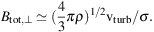 |
(2) |
Application to starlight polarization in the Milky Way yielded field strengths of about 7 µG, in agreement with other methods (Sect. 5). The Chandrasekhar–Fermi method was improved by correcting for the observational errors in polarization angle and signal integration (Hildebrand et al. 2009; Houde et al. 2009; Houde et al. 2011). It can also be applied to radio polarization angles, like in M 51 (Houde et al. 2013).
The Zeeman effect is the most direct method of remote sensing of magnetic fields. In the presence of a magnetic field B∥ along the line of sight, a spectral line is split into two circularly polarized components of opposite sign (longitudinal Zeeman effect). The frequency shift is 2.8 MHz / Gauss for the H I line and larger for molecular lines like OH, CN or H2O (Heiles & Crutcher 2005). The Zeeman effect is sensitive to regular fields, but turbulent fields can also be measured from the dispersion of the circularly polarized signal at a large number of locations on the source (Watson et al. 2001). The interpretation of Zeeman splitting is hampered by its weakness, requiring high line intensities and careful correction of instrumental polarization. Most results have been obtained for the H I line that traces clouds of diffuse (warm) gas in the Milky Way (Crutcher et al. 2010) and for the OH line for starburst galaxies (Robishaw et al. 2008).
Magnetic fields perpendicular to the line of sight generate two shifted lines in addition to the main unshifted line, all linearly polarized (transversal Zeeman effect). These lines cannot be resolved for observations in the Milky Way and external galaxies and no net polarization is observed under symmetric conditions. Detection of linearly polarized lines becomes possible for unequal populations of the different sublevels, a gradient in optical depth or velocity, or an anisotropic velocity field (Goldreich & Kylafis 1981). Depending on the line ratios, the orientation of linear polarization can be parallel or perpendicular to the magnetic field orientation. This Goldreich–Kylafis effect was detected in molecular clouds, star-forming regions, outflows of young stellar systems and supernova remnants of the Milky Way. It was also observed in the ISM of the galaxy M 33 (Li & Henning 2011), where it is consistent with the field orientations along the spiral arms as measured by polarized radio continuum emission (Tabatabaei et al. 2008). The ± 90∘ ambiguity needs to be solved with help of additional continuum polarization data.
3.4. Total radio synchrotron emission and the equipartition assumption
Radio continuum emission from galaxies is a mixture of thermal and nonthermal (synchrotron) components. The average thermal fractions are typically 10% and 25% at 20 cm and 6 cm wavelengths, respectively. At long wavelengths thermal emission is negligible, but thermal absorption may reduce the synchrotron intensity in star-forming regions. A first-order separation of the thermal and nonthermal components can be performed by assuming a uniform spectral index of α = 0.8−1.0 for the nonthermal intensity (I ∝ ν−α) and using the spectral index of the thermal emission in an optically thin plasma of α = 0.1. However, synchrotron intensity depends on energy and age of cosmic-ray electrons (CREs) propagating from the spiral arms and losing energy by synchrotron radiation and inverse Compton scattering with photons, so that the synchrotron spectrum is expected to be flatter (smaller α) in spiral arms than in interarm regions, outer disk and halo. The advanced method to separate the two components introduced by Tabatabaei et al. (2007) uses an extinction-corrected Hα image as a template for the thermal radio emission and was first applied to the galaxy M 33. Simplified separation methods use an Hα image (Heesen et al. 2014) or a combination of Hα and 24 µm infrared images as a thermal template that is subtracted from the total emission (Basu & Roy 2013).
The intensity of total synchrotron emission (examples in Figs. 11, 15, 16, 18 – 20 and 23 – 21, all of which show mostly synchrotron emission) is a measure of the number density of cosmic-ray electrons (CREs) in the relevant energy range and of the strength of the total magnetic field component Btot,⊥ perpendicular to the line of sight (i.e. in the sky plane). Synchrotron emission at a frequency ν is emitted by a range of CREs with average energy E (in GeV) in a field of strength Btot,⊥ (in µG):
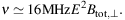 |
(3) |
Equipartition is expected between the energy densities of the total cosmic rays (dominated by protons) and the total magnetic field. The cosmic-ray energy density is determined by integrating over their energy spectrum. This allows us to calculate the total magnetic field strength from the synchrotron intensity (Beck & Krause 2005; Arbutina et al. 2012). The synchrotron intensity Isyn scales with the total magnetic field strength as Isyn ∝ Btot,⊥ 3 + α. Vice versa, Btot,⊥ scales as:
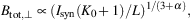 |
(4) |
where α is the synchrotron spectral index (Isyn ∝ ν−α) and L is the effective pathlength through the source. K0 is the ratio of number densities of CR protons and electrons. K0 ≃ 100 is a reasonable assumption in the star forming regions of the disk (Bell 1978). For an electron-positron plasma, e.g. in jets of radio galaxies, K0 = 0. The input parameters, especially the pathlength L and the ratio K0 are not well constrained. Changing one of these values by a factor of e.g. 2 changes the field strength only weakly by 21/(3 + α) ≃ 1.2.
Issues with the equipartition estimate are:
(1) Eq. 4 can be applied only for steep radio spectra with α > 0.5. For flatter spectra, the integration over the energy spectrum of the cosmic rays has to be restricted to a limited energy interval.
(2) Due to the highly nonlinear dependence of Isyn on Btot,⊥, the average equipartition value Btot,⊥ derived from synchrotron intensity is biased towards high field strengths and hence is an overestimate if Btot varies along the line of sight or across the telescope beam (Beck et al. 2003). For α = 1 and the equipartition case, the overestimation factor g of the total field is (see Appendix A in Stepanov et al. (2014)):
 |
(5) |
where < > indicates the averages along the line of sight and the beam, and Q = (<δ Btot,⊥2>)1/2 / <Btot,⊥> is the amplitude of the field fluctuations relative to the mean field. For strong fluctuations of Q = 1, the overestimation factor is 1.46.
(3) If energy losses of CREs are significant, especially in starburst regions or massive spiral arms, the equipartition values are lower limits and are underestimated. The ratio K increases because energy losses of aging CREs are much more severe than those of cosmic-ray protons. Using the standard value K0 underestimates the total magnetic field by a factor of (K / K0)1/(3 + α) in such regions (Beck & Krause 2005). The same applies to the outer disk and halo of a galaxy, where the emitting CREs propagated far away from the places of origin and energy losses are significant.
(4) In dense gas, e.g. in starburst regions, secondary positrons and electrons may be responsible for most of the radio emission via pion decay. Notably, the ratio of protons to secondary electrons is also about 100 for typical radio wavelengths (Lacki & Beck 2013).
(5) Energy equipartition needs time to develop and hence is not valid on small scales in time and space. A correlation analysis of radio continuum images from the Milky Way and the nearby galaxy M 33 by Stepanov et al. (2014) showed that equipartition does not hold on scales smaller than about 1 kpc, which is understandable in view of the typical propagation length of CREs away from their sources (Sect. 4.3). The equipartition field strength is underestimated in regions around the CRE sources and overestimated in regions far away from the sources.
Arguments for the validity of equipartition on large (kpc) scales come from the joint analysis of radio continuum and γ-ray data, allowing an independent determination of magnetic field strengths, e.g. in the Milky Way (Strong et al. 2000), the Large Magellanic Cloud (LMC) (Mao et al. 2012) and in M 82 (Yoast-Hull et al. 2013) 2. Furthermore, the estimates of strengths of large-scale ordered fields derived from Faraday rotation data are similar to those from equipartition in several galaxies (see Table 2 in Van Eck et al. 2015).
3.5. Polarized radio synchrotron emission
Linearly polarized synchrotron emission (examples in Figs. 5, 7, 13, 17 and 22) emerges from CREs in ordered fields in the sky plane. As polarization angles are ambiguous by 180∘, they cannot distinguish regular fields, defined to have a constant direction within the telescope beam, from anisotropic turbulent or tangled fields. Unpolarized synchrotron emission indicates isotropic turbulent or tangled fields that have random directions in 3D and have been amplified by turbulent gas flows (see Sect. 3.1).
The intrinsic degree of linear polarization p0 of synchrotron emission in a perfectly regular field is:
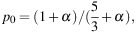 |
(6) |
where α is the spectral index of the synchrotron emission. In spiral galaxies, typical values are α = 0.8−1.0, so that p0 = 73−75%.
The observed degree of polarization is smaller than p0 due to the contribution from unpolarized thermal emission, wavelength-dependent Faraday depolarization (Sect. 3.7) and wavelength-independent “beam depolarization” that is discussed in the following.
Turbulent magnetic fields in galaxies preserve their direction over a coherence scale that depends on the properties of turbulence. 3 In the case of isotropic turbulent fields with a constant coherence length d, the observable degree of synchrotron polarization is (see Sokoloff et al. 1998 for a detailed discussion):
 |
(7) |
where N ≃ D2 L f / d3 is the number of synchrotron-emitting turbulent cells with diameter d and filling factor f within the volume defined by the telescope beam with the linear size D at the galaxy's distance and pathlength L through the source. Eq. (7) is valid only at short radio wavelengths, where Faraday depolarization is small.
Typical degrees of synchrotron polarization observed in nearby galaxies between 3 cm and 6 cm wavelengths with typical spatial resolutions of D ≃ 500 pc are 1−5% in spiral arms (where isotropic turbulent fields dominate), e.g. in NGC 6946 (Beck 2007) and in M 33 (Tabatabaei et al. 2008). With L ≃ 1000 pc and f ≃ 0.5 for the turbulent field coupled to the warm diffuse gas, we get d ≃ 50 pc, consistent with estimates from Faraday depolarization at long wavelengths (Eq. 14).
If the medium is pervaded by an isotropic turbulent field Biso plus an ordered field Bord (regular and/or anisotropic turbulent) that has a constant orientation in the volume observed by the telescope beam, the wavelength-independent polarization (for the case of equipartition between the energy densities of magnetic field and cosmic rays) amounts to (Sokoloff et al. 1998):
 |
(8) |
where q = Biso,⊥ / Bord,⊥ and Biso,⊥ = √2/3 Biso.
3.6. Faraday rotation and Faraday Synthesis
The polarization plane is rotated in a magnetized thermal plasma by Faraday rotation. As the rotation angle is sensitive to the sign of the field direction, only regular fields give rise to Faraday rotation, while the Faraday rotation contributions from turbulent fields largely cancel along the line of sight. Measurements of Faraday rotation from multi-wavelength observations (examples in Figs. 12 and 14) yield the strength and direction of the average regular field component along the line of sight. If Faraday rotation is low (in galaxies typically at wavelengths shorter than a few centimeters), the B–vector of polarized emission gives the intrinsic field orientation in the sky plane, so that the magnetic pattern can be mapped directly (Sect. 4.5).
The Faraday rotation measure RM is defined as the slope of the observed variation of the polarization rotation angle χ with the square of wavelength λ:
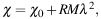 |
(9) |
where χ0 is the intrinsic polarization angle. λ is measured in meters and RM in rad m−2. RM is constant if χ is a linear function of λ2, e.g. if one or more Faraday-rotating regions are located in front of the emitting region (Faraday screen).
A nonlinear variation of χ with λ2 and hence a variation of RM with λ2 occurs in case of:
(1) emission and rotation in the same region where the distribution of electrons or regular magnetic field strength along the line of sight is not symmetric, or field reversals occur, or the field is helical (Sokoloff et al. (1998)),
(2) Faraday depolarization (Sect. 3.7),
(3) several distinct emitting and rotating regions with different contributions to Faraday rotation are located within the beam or along the line of sight or within the source (internal structure).
In these cases, RM needs to be replaced by the Faraday depth Φ (Burn 1966):
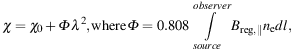 |
(10) |
where Φ is measured in rad m−2, the line-of-sight magnetic field Breg,∥ in µG, the thermal electron density ne in cm−3 and the line of sight l in pc.
To measure the contribution of various sources to Φ, wide-band, multi-channel spectro–polarimetric radio data are needed. These are Fourier-transformed by a software tool called RM Synthesis (Brentjens & de Bruyn 2005; Heald 2015) or Faraday Synthesis (following the terminology proposed by Sun et al. (2015)), to obtain the Faraday spectrum F(Φ) (previously called Faraday dispersion function) at each position of the radio image. F(Φ) shows the intensity of polarized emission and its polarization angle as a function of Φ (Fig. 2).
 |
(a) Sketch of different components along the line of sight. Some of them are emitting (Ei), are Faraday-rotating (Ri), or both. |
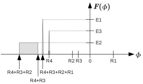 |
(b) Resulting Faraday spectrum F(Φ), where Φ is the Faraday depth, of the components depicted in 2(a). |
Figure 2. Example for a set of different polarization-emitting and rotating components along the line of sight and the resulting Faraday spectrum F(Φ). E1 and E3 are point sources, E2, R2 is an extended emitting and rotating region. R1, R3, and R4 are Faraday screens that are not emitting. Faraday depolarization effects are neglected here for simplicity (from Gießübel et al. 2013). |
If the medium has a relatively simple structure, Faraday spectra at several positions can reveal the 3D structure of the magnetized interstellar medium (Faraday tomography). For example, regular fields, field reversals and turbulent fields can be recognized from their signatures in Faraday spectra (Bell et al. 2011; Frick et al. 2011; Beck et al. 2012b). Helical fields can also imprint characteristic features in the Faraday spectrum (Brandenburg & Stepanov 2014; Horellou & Fletcher 2014). Realistic galaxies have complicated Faraday spectra, as revealed from simplified galaxy models (Ideguchi et al. 2014).
Crucial to successful application of Faraday Synthesis is that the observations cover a wide range in λ2, giving high resolution in Faraday spectra. Even for a wide frequency coverage, two components with a difference in intrinsic polarization angle of about 90∘ cannot be properly recovered by Faraday Synthesis, so that model fitting to the data in Stokes Q and U is needed (Farnsworth et al. 2011).
A grid of RM measurements of polarized background sources is another powerful tool to measure magnetic field patterns in galaxies (Stepanov et al. 2008; Mao et al. 2012). At least 10 RM values from sources behind a galaxy's disk are needed to recognize a simple large-scale field pattern if the Galactic foreground contribution is constant and the background sources have no intrinsic contributions to RM.
Measuring the strength of the regular field from RM needs additional information about the thermal electron density, e.g. from the arrival times of pulsar signals that are delayed in a cloud of ionized gas proportional to the dispersion measure DM = ∫ne dl. The ratio
 |
(11) |
allows us to compute the field strength Breg,∥ (in µG) if the fluctuations in field strength and in electron density are uncorrelated. The value for Breg,∥ derived from pulsar data is an underestimate if small-scale fluctuations in field strength and in electron density are anticorrelated, as expected for local pressure equilibrium, while it is an overestimate if the fluctations are correlated, as expected for compression by shock fronts or turbulence (Beck et al. 2003).
In a single region containing CREs, thermal electrons and purely regular magnetic fields, wavelength-dependent Faraday depolarization occurs because the polarization planes of waves from the far side of the emitting layer are more rotated than those from the near side. This effect is called differential Faraday rotation. For one single layer with a symmetric distribution of thermal electron density and field strength along the line of sight the degree of polarization is reduced to (Burn 1966; Sokoloff et al. 1998):
 |
(12) |
where RM is the observed rotation measure from the source, which is half of the Faraday depth Φ through the whole layer. p varies periodically with the square of wavelength.
Applying Faraday Synthesis (Sect. 3.6) to polarization data of a region that is emitting and Faraday-rotating reveals an extended component in the Faraday spectrum (Fig. 2). However, regions broader than Φmax ≃ π / λmin2 cannot be recovered, where λmin is the minimum wavelength of the observations (Brentjens & de Bruyn 2005); only two “horns” remain visible at the edges of the structure in the Faraday spectrum F(Φ) (Beck et al. 2012b). This problem is similar to the missing short baselines in synthesis imaging.
For multiple emitting + rotating layers, the Faraday spectrum contains several extended components and Eq. (12) is no longer applicable. Shneider et al. (2014) extended Burn's model to a multi-layer (e.g. galaxy disk + halo) medium.
Faraday rotation in helical fields has a completely different behaviour and may lead to an increase of the degree of polarization with increasing wavelength (“re-polarization”) in certain wavelength ranges (Sokoloff et al. 1998; Brandenburg & Stepanov 2014; Horellou & Fletcher 2014).
Turbulent fields also cause wavelength-dependent depolarization, called Faraday dispersion (Sokoloff et al. 1998; Arshakian & Beck 2011). For an emitting and Faraday-rotating region (internal dispersion) the degree of polarization is reduced to:
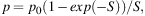 |
(13) |
where S = 2 σRM2 λ4. σRM is the dispersion in rotation measure and depends on the turbulent field strength along the line of sight, the turbulence scale, the thermal electron density, and the pathlength through the medium.
Depolarization by external dispersion occurs in a turbulent Faraday-rotating (but not emitting) medium in the foreground if the diameter of the telescope beam at the distance of the screen is larger than the turbulence scale:
 |
(14) |
An important effect of Faraday dispersion is that the interstellar medium becomes “Faraday thick” for polarized radio emission beyond a certain wavelength, depending on σRM, and only a front layer remains visible in polarized intensity. Typical values for galaxy disks are σRM = 20−100 rad m−2, while star-forming regions can have dispersions of σRM ≃ 1000 rad m−2 (Arshakian & Beck 2011). The maximum in the spectrum of polarized intensity falls into the wavelength range 2–20 cm.
In a random-walk approach, we may write σRM = 0.808 Biso,∥ ne d N∥1/2 (Beck 2007), where Biso,∥ = √1/3 Biso is the strength of the isotropic turbulent field, ne is the electron density within a cell of size d, and N∥ = L f / d is the number of cells along the line of sight L with a volume filling factor f. The average electron density along the line of sight is <ne> = ne / f, so that we get:
 |
(15) |
The average value for galaxy disks of σRM ≃ 50 rad m−2 is consistent with typical values for the warm diffuse ISM of <ne> ≃ 0.03 cm −3 and f ≃ 0.5 (Fig. 10 in Berkhuijsen et al. 2006), Biso ≃ 10 µG, L ≃ 1000 pc, and d ≃ 50 pc.
The dispersion σRM leads to a “Faraday forest” of N components in the Faraday spectrum. If N is not large, the components are possibly resolvable with very high Faraday resolution, hence a wide λ2 span of the observations (Beck et al. 2012b; Bernet et al. 2012).
2 but probably not in NGC 253 (Yoast-Hull et al. 2014) Back.
3 The degrees of polarization expected from compressed or sheared fields are discussed in the Appendix of Beck et al. (2005). Back.