


Star formation takes place in the interstellar medium (ISM), the thin and usually hot gas which occupies much of the volume of most galaxies. The mean free paths of ions, atoms and molecules in the ISM tend to be small compared with the sizes of the structures which they belong to. It is therefore reasonable to approximate the ISM as a smoothly–varying fluid. However, in order to model the behaviour of a fluid on a computer, it is necessary to discretise it in some way into individual fluid elements. How the discretisation is done inevitably has some effect on how physical processes are treated. A very brief summary of the three main types of astrophysical hydrodynamics codes and their advantages and disadvantages is therefore necessary before specific feedback algorithms are discussed. Since this review covers simulations of star formation, particular attention will be paid for each type of code to the way in which the formation of individual stars is modelled.
Grid codes break fluids up into volume elements which fill the space inside a set of boundaries delimiting the computational domain. The simulation is evolved by calculating the forces on the fluid in each volume element and moving material to or from that element's adjoining neighbours. Matter which crosses one of the boundaries is either destroyed (open or outflow boundaries), sent back into the domain as though bouncing off a wall (reflective boundaries), or reinserted at the opposite side of the domain (periodic boundaries). Material may also be created at the boundaries and allowed to flow into the domain (inflow boundaries). Some codes make do with a single fixed grid, but most allow a given grid cell to be subdivided or refined if higher resolution is required at that location, or incorporated into larger grid cells if the resolution at that place is higher than needed. Codes such as flash (Fryxell et al., 2000) and ramses which are able to do this on the fly are known as Adaptive Mesh Refinement codes.
The hydrodynamic equations themselves are solved by a wide variety of methods. Finite difference methods discretise the differential equations connecting quantities in adjacent cells. Finite volume methods integrate quantities over the volumes of the grid cells to compute fluxes between them, often by solving the Riemann problem. Exhaustive reviews of these various methods can be found in many textbooks, e.g. Bodenheimer et al., (2007).
The advantages of grid codes include being able to use virtually any criterion to decide when and where to refine or derefine the grid, and that the mass contained in individual grid cells may become very small or very large, so that very large dynamic ranges in the masses of objects are possible. Disadvantages are that some form of boundary condition must be specified, which limits the volume that can be studied, all grid cells must contain non–zero quantities of gas, so that some computational power may be wasted on simulating regions where very little is happening, and that fluid advection is almost inevitably slightly more efficient along the principal grid axes, leading to artefacts (often known as ‘carbuncles'). Tracing fluid flows in grid codes can be done by advecting passive scalars, but this is somewhat cumbersome and cannot be used to trace completely arbitrary flows. Modelling gravity in grid codes is non–trivial and is usually done by solving Poisson's equation using multigrid methods, although there are also implementations of tree algorithms similar to those used in particle–based codes. In addition, grid codes are not Galilean invariant and moving objects through the grid at speeds in excess of the local sound speed can lead to problems such as unphysical diffusion.
If it occurs that the density of any particular grid cell becomes so high that its integration time becomes prohibitively short, some of the mass in the cell may be converted into a Lagrangian sink particle which is allowed to move between grid cells and to accrete further material. Federrath et al., 2010 describe in detail their implementation of sink particles in flash. As with SPH codes, the first criterion is that the density of the grid cell in question must exceed a given threshold. Six tests are then applied for all cells within a sink accretion radius of the dense cell: (i) the cells must all be on the highest allowed AMR refinement level; (ii) the flow at that location must be converging; (iii) the densest cell must lie at a local potential minimum; (iv) the gas within the accretion radius must be Jeans unstable; (v) the gas within the accretion radius must be bound; (vi) the volume must not overlap the accretion volume of a pre–existing sink. Once a sink is created, it may later accrete gas above the threshold density in the grid cell in which it finds itself, provided that gas is bound to it.
Particle codes discretise fluids into mass elements with a total mass equal to that of the whole fluid. The fluid is evolved by calculating the forces on each particle and moving the particles relative to one another. Since the particles can in principle go anywhere, it is not obligatory to have boundaries of any kind in a particle simulation, although reflective and periodic boundaries are commonly used. Open boundaries at which particles are destroyed, or inflow boundaries where new particles are inserted are also possible but uncommon.
By far the most popular particle method is Smoothed Particle Hydrodynamics (SPH, e.g. Springel, 2010b). SPH codes represent fluids as particles whose masses are smoothed or smeared out over a volume called the smoothing kernel. The kernel is spherical, but the smoothing is done such that most of the mass is concentrated near the particle centre. The radius of the smoothing kernel is continuously recomputed so that it contains the centres of, on average (or, in some codes, exactly) a given number (usually ≈ 50) of ‘neighbour' particles. This is achieved in many codes (e.g. seren, Hubber et al., 2011) by iteratively solving for each particle i the expression ρi hi3 = constant (i.e. the fixed particle mass), as described in Springel, (2010b). Fluid quantities such as density are computed as averages over a particle and all of its neighbours. The requirement that the number of neighbours be fixed automatically results in the smoothing kernels, which set the resolution of an SPH code, being smallest where the gas density is highest.
Gravitational forces could in principle be computed directly between particles, but this scales extremely poorly as the number of particles increases so is rarely if ever used. Many codes reduce the expense of computing the gravitational forces by grouping particles into a tree structure, and computing gravitational forces using tree nodes instead of individual particles, provided that the tree node subtends a sufficiently small angle at the location where the forces are to be computed. Alternatively some codes use the particle–mesh method where the particle densities are converted to densities on a mesh and gravitational forces are computed by solving Poisson's equation.
Not needing boundaries, the relative ease of computing self–gravitational forces, and the possibility of having parts of the computational domain genuinely empty are the main advantages of particle codes. Since each particle has a unique and preserved identity, it is also trivial to trace fluid flows in particle simulations, which is very helpful when, for example, studying triggered star formation or pollution by supernovae. Particle codes generally do not treat shocks as well as grid codes, and they are restrictive in the sense that only the mass density can be used to control the resolution and other quantities cannot be refined on as needed. Traditionally, particle code also have problems dealing with contact discontinuities Agertz et al., 2007), although there are now several solutions to this issue available (e.g. Read et al., 2010, Saitoh and Makino, 2013).
Since they are Lagrangian codes, implementing sink particles in SPH schemes is somewhat more straightforward than in grid codes, since the sinks can be treated like gas particles except that they do not feel or exert pressure forces. An early implementation was described by Bate et al., (1995). A density threshold is defined and any gas particles exceeding this threshold, along with their neighbours, are considered for sink formation. Four criteria must be met: (i) the ratio α of thermal to gravitational potential energy of the group must be < 0.5 (ii) the sum of α and β, the ratio of rotational energy to gravitational potential energy must be < 1 (iii) the total energy of the group must be negative (iv) the divergence of the acceleration must be negative. If these tests are passed, a sink is created with the total mass and momentum of the seed gas particles.
Accretion onto the sink is achieved by assigning it an accretion radius and testing particles which pass within it. Particles which are bound to the sink with a specific angular momentum less than that required to form a circular orbit at the accretion radius are accreted. A much more sophisticated SPH sink particle algorithm was recently presented by Hubber et al., (2013). The creation criteria are again that the gas particle being considered for promotion must have a density exceeding a threshold, the putative sink particle would not overlap any pre–existing sinks, it must sit at a local potential minimum, and the candidate particle's density must be such that it is smaller than the Hill sphere defined by itself and any pre–existing sink.
Once created, their sinks do not immediately accrete gas particles entering the accretion radius (which they term the ‘interaction zone'). Instead they are added to an interaction list (from which they may be struck off if they exit the interaction zone) and are gradually accreted over a physically–motivated timescale, while still being permitted to interact with other SPH particles. The smooth accretion and the continued interaction with gas particles outside the sink interaction zone, particularly in respect of angular momentum transfer, results in more physically–motivated and robust sink behaviour.
In practice, most of these conditions are usually dropped in large–scale simulations where sink masses are too big for them to considered as single stars. In these cases, sink particles are often created simply from particles whose densities exceed a threshold.
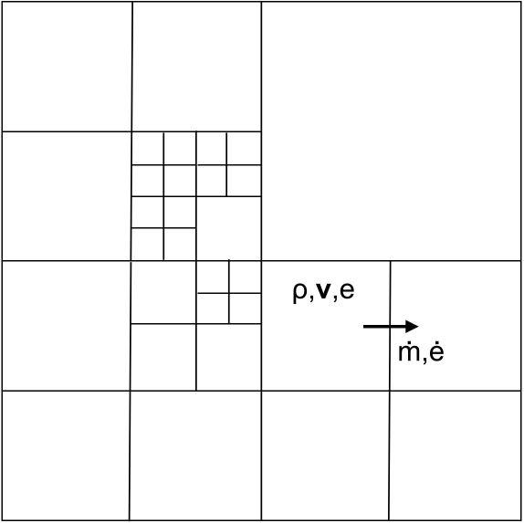
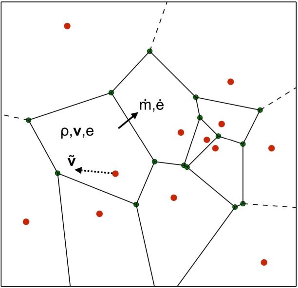
The most recent additions to the stable of astrophysical fluid codes are the moving–mesh codes (e.g. Gaburov and Nitadori, 2011, Hopkins, 2015). The most widely used to date is arepo (Springel, 2010a) which solves the hydrodynamical equations using a finite–volume Godunov method on a 3D Voronoi mesh dynamically created around a population of Lagrangian particles which follow the fluid flow. The code is then in some sense a hybrid between traditional grid– and particle–based codes, and shares most of the advantages and few of the drawbacks of both alternatives. Moving–mesh codes are Galilean–invariant like SPH codes but capture shocks and contact discontinuities as well as grid codes. They also share the ability to refine or derefine their resolution based on arbitrary conditions by splitting or merging their Lagrangian tracer particles. Sink particles can be implemented in ways analogous to those employed by grid–based codes, in which sinks remove mass from grid cells. The only disadvantages of moving–mesh codes are their relative complexity and novelty. Figure 1 illustrates schematically the differences between these three types of code.
 |
 |
 |
| (a) SPH | (b) AMR | (c) Moving mesh |
Figure 1. Simple illustration of the ideas behind the major types of astrophysical hydrodynamics code. The left panel shows how an SPH code represents a fluid, with red dots being individual particles carrying a mass m and specific internal energy u. Each particle has a velocity v and feels forces from other particles. Denser regions of gas are represented by higher concentrations of particles. The size of a particle is defined by the radius 2h which encloses a constant number of neighbours (here, only 4 for clarity). The middle panel shows an AMR representation of a fluid with only three levels of refinement. The gas in each cell has a density ρ, velocity v and internal energy e. Cells exchange mass, momentum and energy with their neighbours. The right panel depicts a moving mesh code. The fluid mass is again represented by particles, shown as red dots, and the fluid volume is partitioned around these by a Voronoi tessellation. Cells exchange matter, momentum and energy, but the particles move with the fluid flow. |
||