4. FEEDBACK ALGORITHMS

This section briefly surveys some of the algorithms used to model stellar feedback mechanisms. The focus is on the algorithms themselves and the assumptions that underlie them. The results gained from using them will be discussed in a later section.

4.1. Radiative transfer algorithms

During and after their formation, stars – even low–mass objects – are strong sources of radiation which deposit energy and momentum into the surrounding gas. The interaction of radiation and matter is an immensely difficult problem to solve and a great deal of effort has been expended on it. The summary given here is of necessity brief – a more detailed and wide–ranging review can be found in Trac and Gnedin, (2011). The two main processes of interest here are the radiation emitted mostly in the infrared by protostars (deriving from the loss of gravitational potential energy by accreting material and by the contracting protostar itself, and sometimes due to the burning of deuterium before hydrogen burning gets underway), and emission of ultraviolet photoionising photons by massive stars as they quickly settle onto the main sequence.

In common with self–gravitational forces, radiative transfer (RT) in principle allows every part of the computational domain to communicate with every other part. However, the latter issue is much worse, since the communication between any two fluid elements depends on all the intervening material through which any radiation must pass, which of course does not apply to gravitational forces. This problem is in general too demanding to be solved explicitly but numerous physical and numerical approximations have been made to render it tractable.

4.1.1. Ray–tracing methods

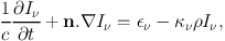
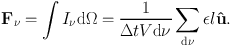
The most intuitive approach to RT computations is ray–tracing, that is, drawing lines from radiation sources to target fluid elements and solving the radiation transfer equation along them. We shall limit ourselves to the consideration of unpolarised radiation. The time–dependent RT equation takes the form

(5)

with I_ν the specific intensity at frequency ν, n a unit vector pointing in the direction of radiation propagation, є_ν the emissivity of the medium and κ_ν the specific absorption coefficient. This is an equation in seven variables and solving it is a formidable problem. This is particularly true if large frequency ranges are of interest, for which the frequency dependence of the emissivity and opacity is likely to be significant and the problem has to be solved for many different values of ν. It is common to avoid this issue by computing effective average emissivities and opacities, commonly referred to as the ‘grey' approximation.

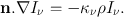
It is also common to simplify Equation 5 by various approximations. If the time–dependence can be neglected, equivalent to finding a radiative equilibrium, the time–independent RT equation results:

(6)

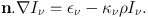
Furthermore, it is often the case that the radiation field is dominated by a small number of very bright sources (e.g. stars), and that the emissivity of the gas may be neglected, yielding

(7)

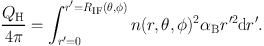
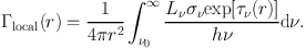
Several authors have made use of ray–tracing algorithms to attack the problem of photoionisation, differences being mainly in how they choose to cast their rays. Under the OTS approximation, any number of independent rays may be drawn emanating from an ionising source and the thermodynamic state of the gas can be found by locating the ionisation front along each ray using a generalisation of Equation 1. If the radius of the ionisation front is a function of direction R_IF(θ, φ), one can write

(8)

Kessel-Deynet and Burkert, (2000) and Dale et al., (2007c) using SPH codes defined rays connecting the ionising source to all active gas particles (a similar method was used by Johnson et al., (2007), except they first constructed a spherical grid with 10⁵ rays, each divided into 500 radial segments). Particles' neighbours are tested to find the one closest (in an angular sense) to the ray leading back source. This process is repeated until the source is reached, generating a list of particles along the ray, whose densities are then used to calculate the integral in Equation 8. This can be used in a time–independent way to locate the ionisation front assuming ionisation equilibrium and heat the gas behind the ionisation front. However, Dale et al., (2007c) use it to compute the photon flux at each particle to determine whether it is sufficient to keep an ionised particle in that state, or to (partially or completely) ionise a neutral particle, during the current timestep.

This algorithm was modified in Dale and Bonnell, (2011) and Dale et al., (2012b) to allow for multiple sources ionising the same HII regions. In the former paper, this was achieved by identifying all particles illuminated by more than one source and dividing their recombination rates by the number of sources illuminating them. The solution for the radiation field is iterated until the number of ionised particles converges. In the latter paper, a more sophisticated approach was adopted where the total photon flux at each particle is evaluated and the fraction of the recombination rate that each source is expected to pay for at a given particle is set by the flux striking it from that source as a fraction of the total. These methods give similar results in practice.

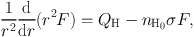
In the Eulerian heracles code by Tremblin et al., (2012b), solve a differential form of Equation 8, taking the photon flux F as the variable of interest, writing

(9)

where σ is the absorption cross section to ionising photons and n_H0 is the density of neutral hydrogen atoms. This equation is then complemented with equations describing photochemistry. The ionisation fraction x is n_H⁺ / n_H and n_H = n_H⁺ + n_H0. The number of photons absorbed in a grid cell of volume dV_cell is given by the flux of photons entering the cell through the surface dA multiplied by the probability of absorption dP = σ n_H0 ds, with ds being the pathlength along the ray. This allows one to write

(10) (11) (12)

where the last term in the last equation is a geometrical dilution factor. Once these equations have been solved, the heating due to the absorption of ionising photons and the cooling due to recombinations can be computed.

Gritschneder et al., (2009a) modelled the propagation of plane–parallel ionising radiation in SPH. Rather than drawing rays to every particle, they used an adaptive scheme, casting a small number of rays along the photon propagation direction, and recursively refining them into four subrays up to five times at locations where the separation of the rays exceeded the particle smoothing lengths.

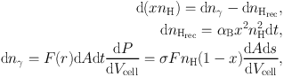
Similarly, but in spherical geometry, Bisbas et al., (2009) used the HEALPix tessellation (Górski et al., 2005) to define rays, starting with the lowest level and refining rays into four subrays. Rays are refined when their separation, given by the radius r_ray at which they are defined multiplied by the separation angle θ_l of the HEALPix level l to which they belong, exceeds the local smoothing smoothing length h multiplied by a parameter f₂ of order unity. Values of f₂ of 1.0–1.3 were found to give a reasonable compromise between speed and accuracy.

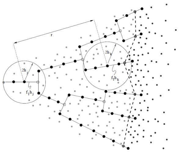Figure 2. Schematic representation of the adaptive SPH ray–tracing technique employed by Bisbas et al., (2009). The ionising source is represented by the star at the extreme left. Solid lines are rays, with black circles representing the evaluation points used to compute the discrete integral Equation 8. Grey circles are locations where they rays are split into four sub rays. The dashed line beyond which the particle density becomes abruptly larger is the ionisation front.

Once rays are defined, the discrete integral in Equation 8 is computed along them by defining a series of evaluation points, each being a distance f₁h from the previous one, with f₁ a dimensionless factor (given a value of 0.25) and h being the local smoothing length. A schematic is shown in Figure 2. The ionisation front is linearly smoothed over one smoothing length and the gas heated accordingly. A smiler adaptive ray–tracing scheme was presented by Abel and Wandelt, (2002) for use on Cartesian grids. This scheme differs from that of Bisbas et al., (2009) in that child rays can be merged in regions where high resolution is not necessary, and that they solve a time–dependent problem, using the results of the ray–trace to compute fluxes at cells. The algorithm is taken even further by Wise and Abel, (2011), who also implement non–ionising radiation (e.g. Lyman–Werner dissociation) and radiation pressure.

Krumholz et al., (2007b) use a variant of the ray–tracing method of Abel and Wandelt, (2002), periodically rotating the rays with respect to the Cartesian grid to avoid geometrical artefacts. To avoid spurious overcooling at the ionisation front, molecular heating and cooling processes are disabled for cells with ionisation fractions in the range [0.01,0.99]. They also explore the convergence of the results with changes in the update timestep for the radiation scheme, which effectively sets by how much the temperature of a cell near the ionisation front is allowed to change in one timestep. Allowing the temperature to change by a factor of 100 led to larger errors in the location of the ionisation front at early times, although the error declines as the front expands, and they caution against allowing sudden temperature jumps in photoionisation algorithms. This was also pointed out by Whalen and Norman, (2008), who explicitly compared an algorithm employing the assumption of ionisation equilibrium embodied by Equation 8 with a more sophisticated radiative transfer algorithm described in Whalen and Norman, (2006). They found that the structure of ionisation–front instabilities varied substantially between the two codes, especially at early times, and attributed the differences to the sudden heating inherent in the equilibrium method.

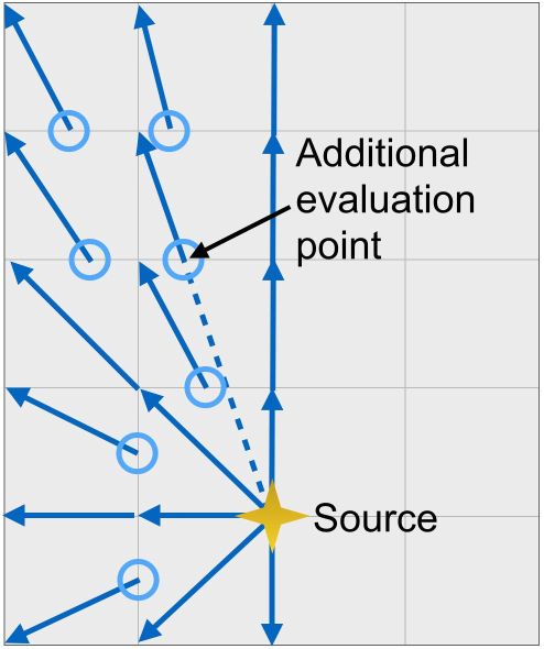
Peters et al., (2010) implemented the ray–tracing algorithm of Rijkhorst et al., (2006) in the flash AMR code (Fryxell et al., 2000). The algorithm computes column densities on nested grids using a hybrid long– and short–characteristics method. A long characteristic is a ray drawn between a radiation source and an arbitrary cell, and may have many segments since it may pass through many intervening grid cells. A single long characteristic can transport radiation between two arbitrary points in the simulation. A short characteristic passes only across a single grid cell and only transports radiation from one cell to another (see Figure 3 for an illustration). From a computational perspective, long characteristics are more amenable to parallel computation, since each ray can be treated independently and the radiation transport equation solved along it. However, time is wasted near the source, since many rays pass though the same volume. Short characteristics cover the domain uniformly but radiation properties of cells must be updated from the source working outwards because each short characteristic must begin from the (usuallly interpolated) end solution of one closer to the source. Short characteristic methods are therefore difficult to parallelise and more diffusive.

(a)	(b)
Figure 3. Illustration of the difference between long and short characteristics. Long characteristics (left panel) are drawn from the source to every grid vertex, so that regions close to the source are crossed by many rays. Short characteristics (right panel) are drawn across single cells, connecting the point where a vector from the source enters the cell (dotted line) to the nearest grid vertex. The radiation field at the entry points of cells (blue circles) must be interpolated from values at neighbouring vertices, making this method more diffusive.

For a given AMR block, the Rijkhorst et al., (2006) algorithm computes pseudo–short–characteristic rays which enter the block from the direction of the source and terminate at all the cell centres for use local to that block, and pseudo–long–characteristic ray segments which terminate at the cell corners. It is the latter which are shared with other processors so that what are effectively long characteristics can be stitched together across blocks. Once the rays have been defined, transfer of ionising photons is solved in a manner similar to that employed by Tremblin et al., (2012b), save that collisional ionisations are also accounted for.

Several authors (e.g. Mackey and Lim, 2010, Arthur et al., 2011) use the c²–ray algorithm of Mellema et al., (2006b) to model photoionisation feedback. This method is photon–conserving and accurately solves the RT problem in the (common) case that the computational resolution elements are optically thick. For an infinitesimally thin spherical shell of radius r with a radiation source of luminosity L at its centre, the rate of absorption of photons per unit area is

(13)

If, however, the shell has a finite thickness Δr, photons strike the inner surface at a rate (r − Δr/2) and emerge from the outer surface at a rate (r + Δr/2), and the number of atoms in the shell is nV_shell. Equation 13 can then be rewritten as the photoionisation rate across a finite shell,

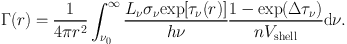(14)

If Δτ_ν tends to zero, Equation 14 reduces to Equation 13. This issue could place severe constraints on the spatial discretisation required to model the propagation of an ionisation front. Mellema et al., (2006b) also discuss issues of time discretisation. The above assumes that the optical depth does not change over the course of the computational timestep, so that either a very small timestep is required, or a time–averaged value of the optical depth should be used. They show that using at any location the time– and space–averaged values of the neutral density, ionisation fraction and the optical depth from the source allows accurate solution using large timesteps, at least as long as the local recombination time, and volume elements with large optical depths.

Clark et al., (2012a) present treecol which solves Equation 7 in an SPH code using the gravity tree to speed up the calculation of optical depths. The idea behind the gravity tree is that when computing the gravitational forces acting on a given particle, groups of particles which are sufficiently far away can be amalgamated into pseudoparticles. The gravity tree groups all particles into a hierarchy, usually by recursively dividing the simulation domain into eight subdomains. When computing gravitational forces, the angle subtended at the particle by all the tree nodes is computed and compared to a parameter θ_c, the tree–opening angle. If the node subtends an angle larger than θ_c at the particle in question, the node is decomposed into its children and they are tested. Once nodes subtending angles smaller than θ_c are found, they are treated as pseudoparticles.

treecol uses this formalism to save time in computing column–densities along rays. For every particle, a low–level (48– or 192–wedge) healpix tessellation is constructed and the contribution of tree nodes to the column density in each wedge is computed, respecting the tree–opening angle criterion. This results, for every particle, in a moderate–resolution map of the column density from its location to the edge of the simulation domain. This is ideal for computing external heating by a radiation bath such as the ambient UV background that permeates the ISM. Bate and Keto, (2015) recently presented a code which hybridises the FLD model of Whitehouse et al., (2005) with a version of treecol to model, respectively, protostellar heating and heating from the intercloud radiation field. A method analogous to treecol but designed specifically for AMR–based trees was recently described by Valdivia and Hennebelle, (2014).

4.1.2. Moment methods

Many alternative approaches to the RT problem involve so–called moment methods. The fundamental radiative quantity is the intensity or spectral irradiance, I_ν which describes at a given location the rate at which energy is emitted per unit area, per steradian and per frequency interval. Integrating over frequency and integrating out the angular dependence yields the zeroth, first and second moments of the radiation field, better known as the energy density E, radiative flux F and the radiation pressure tensor P:

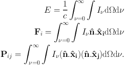(15) (16) (17) (18)

While the meaning of E and F are clear, the radiation pressure tensor needs a little explanation. Its (i, j) component P_ij is the rate at which momentum in the î direction is being advected by the radiation field through a surface whose normal is the ĵ direction.

Once these transformations are done, the radiation field can be treated like a fluid, coupled to the matter density field by the equations of radiation hydrodynamics (RHD). In a frame following the flow of matter and under the assumption of local thermodynamic equilibrium, the RHD equations can be written (Turner and Stone, 2001):

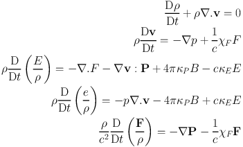(19) (20) (21) (22) (23)

where χ_F is the frequency–integrated mean opacity including components due to absorption and scattering, and κ_P and κ_E are the Planck mean and energy mean absorption opacities, and the colon operator represents a double dot product operation.

A popular approach to solving these equations, owing to its conceptual simplicity, is the flux–limited–diffusion (FLD) method. FLD simplifies the evolution of the radiation flux by first assuming a steady state, so that the derivative on the LHS of Equation 23 vanishes, then asserting that the radiation field is approximately locally isotropic, so that P = E / 3 and

(24)

As the opacity becomes small, this approximation for the radiation flux tends to infinity, whereas in fact F cannot exceed cE. In the optically thin limit, the radiation field can in principle be strongly anisotropic, so that the assumptions behind the derivation of the moment equations break down. However, this problem can overcome by inserting an additional parameter into Equation 24:

(25)

where λ(E) is the flux–limiter, whose purpose is to prevent the energy flux becoming unphysically large. The flux limiter can be defined via the radiation pressure tensor as follows. P can be written in terms of E as P = fE, with f being the Eddington tensor, which simply encodes the local directionality of the radiation field. Formally,

(26)

with = ∇ E / |∇ E|, is a tensor formed by the vector outer product of with itself, and f is the dimensionless Eddington factor. The flux limiter is then defined via f = λ + λ² R², where R = |∇ E| / (χ E). The function λ must then be chosen so that the radiation field is always reconstructed smoothly.

Whitehouse et al., (2005) and Bate, (2009) implemented the effects of accretion heating from low–mass protostars in SPH using the FLD approximation. These models account for conversion of gravitational potential energy to heat in the accretion flows (i.e. it is radiated away in a physical manner as opposed to be being entirely lost, as in an isothermal model, or entirely retained as in an adiabatic model). However, the protostars have no intrinsic luminosity of their own, so that the feedback in these calculations is effectively a lower limit (Offner et al., 2009).

Krumholz et al., (2007a) report on a FLD method implemented in the orion AMR code to model radiative feedback in massive molecular cores, considering sink particles as radiation sources. The detailed protostellar models are derived from McKee and Tan, (2003) and account for dissociation and ionisation of infalling material, deuterium burning, core deuterium exhaustion, the onset of convection and hydrogen burning. They set an opacity floor at high temperatures, since FLD schemes do not deal well with sharp opacity gradients where the radiation field can be strongly anisotropic.

To avoid the issues that can be encountered in FLD with steep opacity gradients, Kuiper et al., (2010) present a novel hybrid method which combines FLD and ray–tracing. They split the radiation field into two components. Diffuse thermal dust emission is computed using an FLD method, whereas the direct stellar radiation field is handled by doing ray–tracing on a spherical grid either in the grey approximation, or using (typically ≈ 60) frequency bins to capture frequency–dependent opacities.

Krumholz et al., (2009) used the orion code with FLD to model accretion onto high–mass protostars. They simulated a 100 M_⊙, 0.1pc radius rotating core which collapsed to form a disc with a central massive object. Once the star achieved sufficient mass, Kelvin–Helmholtz contraction raised its luminosity to the point where radiation pressure became dynamically important. Radiation dominated bubbles inflated along the rotation axis and infalling material landed on the bubbles, travelled around their surfaces and was deposited in the accretion disc. The accretion rate onto the massive star was thus little altered. A second star grew in the disc resulting in a massive binary, and the radiation–inflated bubbles became Rayleigh–Taylor unstable, rapidly achieving a steady turbulent state.

Kuiper et al., (2012a) and Kuiper et al., (2012b) simulated essentially the same problem – accretion onto a high–mass protostar – using their hybrid FLD/ray–tracing approach and arrived at qualitatively different results. In the latter paper, they performed a comparison in which they operated their code using the FLD solver only. Both radiation transport schemes drove radiation–dominated cavities, but those produced by the hybrid scheme continued to grow until leaving the simulation domain, whereas those from the pure–FLD run collapsed along the rotation axis. They found that the cavity in the FLD case was unable to resist accretion onto it, which they attribute to the radiative flux in the FLD method tending to point in directions that minimise the optical depth, allowing photons to escape and depressurising the cavities. The hybrid scheme does not suffer from this problem, because the stellar radiation field is transported by direct ray tracing. They did not observe the kind of instability seen by Krumholz et al., (2009).

A second alternative to FLD is to compute the Eddington tensor directly. These are usually known as variable Eddington tensor (VET) techniques, and differ in the ways they compute or estimate the tensor. Gnedin and Abel, 2001 give a very clear description of the basis of these techniques. They define the VET as f_ij = P_ij / Tr(P_ij) with

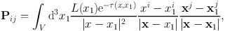(27)

where x₁ are the position vectors of the radiation sources and could consist of a set of δ–functions modelling stellar sources, or could include every point in the domain if diffuse radiation fields are of interest. L(x₁) is the luminosity function of the sources and, x is the location at which the radiation field is to be computed. This integral is very expensive to evaluate because of the optical depth term e^{−τ(x, x₁)}.

Gnedin and Abel, (2001) make the integral tractable by dropping this term. This means that the radiation flux is computed at each point in the simulation domain assuming that the radiation reaching it from all sources suffers only r⁻² geometric dilution, with no opacity effects. This is referred to as the optically thin variable Eddington tensor, or OTVET, scheme. They stress that this latter approximation is not the same as in standard diffusion methods, because in these the Eddington tensor is computed strictly locally. They also point out that radiation need not be propagated at the speed of light, as long as its characteristic velocity is much larger than any dynamical velocities present. They suggest that even 100 km s⁻¹ may be adequate. Schemes making use of this approximation are known as reduced–speed–of–light (RSL) methods. OTVET methods have also been implemented in SPH codes, e.g. Petkova and Springel, 2009 in gadget–3, and Sales et al., (2014) implement an improved version of the Petkova and Springel, (2009) scheme in the arepo code.

Some tension has recently emerged between FLD and OTVET schemes. Davis et al., (2012) use a short–characteristics VET method in athena and perform explicitly comparisons with an FLD solver and a Monte Carlo solver implemented in the same code. The Monte Carlo algorithm is much too slow to be used in a dynamical simulation, so they instead use the three schemes to obtain an equilibrium solution on a single snapshot from a shearing–box simulation. They find that the VET and MC methods agree well, with the FLD solver being the odd one out, with the discrepancies largest in optically–thin regions.

Krumholz and Thompson, (2012) use a two–temperature FLD approximation on a 2D Cartesian grid to study the evolution of radiation pressure driven winds in a gravitationally–stratified atmosphere (intended as an approximation to ULIRGs and bright, dense young star clusters). Simulations are characterised in terms of whether the radiation pressure forces are greater or smaller than the gravitational forces. Where the radiation pressure forces are smaller, the gas undergoes vertical oscillations which eventually die out. Otherwise, an instability resembling the Rayleigh Taylor instability develops, with columns of dense gas falling into the low–density material at the base of the atmosphere where the radiation pressure forces are greatest. These columns contain most of the mass, but the low density and low optical depth gas occupies most of the volume, allowing radiation to escape in the vertical direction. The simulation reaches a steady turbulent state with nearly constant velocity dispersion and density scale height.

Davis et al., (2014) also modelled radiation pressure feedback in ULIRGs. RT was implemented in 2D in the athena code using either FLD or VET, and substantial differences exist between the results. In the low–flux case, both radiative transfer schemes (and Krumholz and Thompson, 2012) agree that the gas undergoes stable vertical oscillations. Their high–flux FLD case rapidly becomes Rayleigh–Taylor unstable, as does that of Krumholz and Thompson, (2012), and most of the gas sinks back towards the z=0 plane, where it remains in a turbulent state. However, in the VET calculation, the behaviour is very different. The RTI also develops, but most of the dense gas is nevertheless accelerated upwards out of the simulation domain. The volume–averaged Eddington factor in the VET run is generally larger than in the FLD run and exceeds unity for most of the time, while in the FLD run it is mostly just under unity. The difference is modest, but crucial. Deeper analysis shows that the two schemes agree well in the dense gas, where FLD should be a good approximation, but disagree on the magnitude and direction of radiation fluxes in low–optical depth regions where the diffusion approximation is likely to fail. In some regions, the FLD fluxes point in the opposite direction to the VET fluxes, accelerating the gas downwards instead of upwards, reinforcing the development of low–density channels and accelerating the development of the RTI.

4.1.3. Monte Carlo methods

Monte Carlo methods solve the RT problem by emitting ‘photon packets' in randomly–chosen directions from the radiation source and following their paths through the simulation domain. In each fluid element through which the packet passes the probability of it being absorbed or scattered is computed and more random numbers are used to decide its fate. This is repeated with a large enough number of packets to sample the radiation field and iterated until some convergence criterion is satisfied. Monte Carlo codes are good at modelling processes such as scattering and re–emission, which are cumbersome to compute in ray–tracing schemes, and covering the frequency domain of the radiation transport problem is relatively simple, although it usually entails emitting more photon packets. The drawback of Monte Carlo methods is that they converge slowly and there is inevitably noise in the resulting temperature field owing to the discrete emission of energy.

Monte Carlo methods are expensive and have traditionally been used to post–process the interaction of non–dynamically–important radiation fields with fixed pre–computed matter density distributions. However, improvements in computer power and algorithms have recently led owners of Monte Carlo codes to implement hydrodynamical algorithms in the codes (the reverse of what is usually done).

The sphray algorithm is presented by Altay et al., (2008). Not a Monte Carlo code in the strict sense, sphray uses the c²–ray method to solve the radiation transport equation on randomly–cast rays in an SPH simulation. All particles through which a ray passes are identified using the Axis–Aligned Bounding Box method acting on an octal tree. In solving the photoionisation problem, the OTS approximation is made (for both hydrogen and helium ionisation). The impact parameters of particles intersected by the ray is computed and the smoothing kernel integrated through accordingly to compute the particle's contribution to the optical depth. Photon packets are then propagated along rays and a fraction of their energy (1 − e^−τ_ν) is subtracted as they pass through each particle.

Pawlik and Schaye, (2008) present the traphic SPH RT code. Radiation packets are emitted from sources every simulation timestep and propagated through the gas until a stopping criterion is satisfied. Each source (which can be a star particle or a gas particle) emits photons into an array of cones that covers the sky. Virtual SPH particles are placed into any cones which do not contain any real gas particles. Photon packets are distributed amongst the real and virtual neighbours of a source, and are then passed on in the radial propagation direction in a cone with the same opening angle as the original emission cone. The cones therefore subtend smaller and smaller solid angles at the source as one moves further away. Gas particles can receive and retransmit multiple photon packets, and packets coming from similar directions are merged to improve efficiency.

Particles absorb energy from photon packets according to their opacities, removing a fraction (1 − exp^−τ) of the energy from the packet. Alternatively, photon packets can be reemitted, treating the gas particle as a radiation source, to model scattering. The absorption and reemission process continues until one of two stopping criteria are reached. If a state of radiative equilibrium is desired, the process is continued until all packets have been absorbed or have left the simulation domain. Otherwise, photon propagation is stopped when the packets have travelled a distance set by the speed of light and the timestep.

Nayakshin et al., (2009) present an algorithm for modelling radiation pressure in SPH using a Monte Carlo method. They track the trajectories of photon packets as r(t) = r₀ + v_phot t, where the propagation speed |v_phot| need not be the speed of the light. They also reduce the packet energies E_phot and momenta p_phot = E_phot / c continuously, rather than discretely, using

(28)

Packets are destroyed when their momentum drops below 10⁻⁴ of its initial value.

Harries, (2011), Haworth and Harries, (2012), Harries, (2015) implemented a grid–based finite volume hydrodynamical scheme into the pre–existing TORUS Monte Carlo code. Photon packets have constant total energy and are initially given a frequency chosen randomly using the source emission spectrum. The frequency determines the number of photons the packet represents. For a source luminosity L, integration time interval Δt and number of packets N, the energy per packet is just є = LΔt / N. The packet propagates in a randomly–selected direction for a randomly–chosen pathlength l, at the end of which it is absorbed. A new packet is immediately emitted at that location in the same fashion, but with a frequency determined by the emission spectrum of the gas at the absorption point. This continues until the packet leaves the grid or its propagation time becomes equal to Δt.

As packets travel through the grid, they contribute to the energy density in every cell through which they pass. Each packet contributes dU which is estimated from

(29)

with V being the cell volume. In the photoionisation calculations presented by Haworth and Harries, (2012), this can be used immediately to solve the ionisation balance equations (Osterbrock and Ferland, 2006). For a given species X with ionisation states Xⁱ, Xⁱ⁺¹, etc., the balance equation reads

(30)

where α(Xⁱ) are recombination coefficients, a_ν(Xⁱ) are absorption cross sections, n_e is the electron number density, and ν₁ is the ionisation threshold frequency for species Xⁱ respectively. torus continues iterating the radiation transfer until an equilibrium temperature is achieved in each cell such that the heating and cooling rates balance. In radiation hydrodynamics calculations, the radiation transport problem is solved by iteration first, since the solutions for subsequent timesteps are likely to be relatively small perturbations on the initial state, and the radiation and hydrodynamics problems are then solved one after the other, with the radiation always being done first.

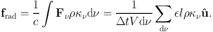
Harries, (2015) discusses two methods by which radiation pressure forces may be computed in Monte Carlo schemes. The simplest is to compute the change in momentum Δp_phot suffered by a packet in a cell and add that impulse to the gas in the cell

(31)

where û_in and û_out are the unit vectors of the packet's trajectory as it enters and leaves the cell respectively. The radiation force can then be computed at the end of the iteration from f_rad = ∑Δp_gas / (Δt V).

The above method suffers problems in optically thin gas, however, where the number of absorptions and scatterings can be small or zero. This can be overcome by computing the radiation pressure directly from the radiation flux. Equation 29 can be rewritten to give an expression for the radiation intensity

(32)

leading to a Monte Carlo estimate of the radiation flux

(33)

The force may be computed by converting the above expression into one for momentum flux and multiplying it by an appropriate opacity ρκ_ν:

(34)

A much smoother estimate of the radiation pressure is recovered by this last expression, since all packets passing through a cell contribute to the estimate, and not just those that are absorbed or scattered.

In principle, Monte Carlo methods are very easy to parellelise, since each photon packet can be treated independently. On a shared memory machine where all the processors can access the entire computational domain, parallelisation is than almost trivial. However, most problems are run on distributed–memory machines using the message–passing interface (MPI). The moccasin code (Ercolano et al., 2003) gets around this problem by giving a copy of the whole domain to each processor, but this is very memory intensive and it is more usual to decompose the domain into subdomains, as is done in torus. When a photon packet leaves one sub–domain belonging to one processor for another belonging to a second processor, the first processor sends an MPI message containing the details of the packet to the second. In torus, photon packets are communicated in stacks to cut down on communication overhead.

4.1.4. Alternative methods

Stamatellos et al., 2007 devised a novel method for estimating the mean optical depth at the location of an SPH particle from the local density, temperature and gravitational potential, reasoning that the optical depth and the gravitational potential are both non–local properties determined by each particle's location within the simulation as a whole. Each particle is regarded as being inside a spherically symmetric polytropic pseudo–cloud at an unspecified location. For any location within the pseudocloud, the central density and scale length are adjusted to reproduce the actual density and potential (neglecting any stellar contribution) at the SPH particle's location within the real gas distribution. The optical depth for any given location is computed by integrating out along a radius to the edge of the pseudo–cloud. The target particle is then allowed to move anywhere in the pseudo–cloud and a mass–weighted average optical depth over all possible positions is computed. Radiation transport is then conducted in the diffusion approximation.

Another approach, taken for example by Urban et al., (2009), is to treat the detailed radiation transport problem as subgrid physics, and to parameterise it in some way. Urban et al., (2009) used detailed one–dimensional dusty (Nenkova et al., 2000) models or analytic one–dimensional approximations to compute the temperature distribution near protostars owing to their accretion and intrinsic luminosities, and imprint the temperatures on their 3D SPH simulations.

MacLachlan et al., (2015) use the mcrt Monte Carlo RT code (Wood et al., 2004) in a novel way to essentially post–process the galactic–scale dynamical simulations of Bonnell et al., (2013). Snapshots from the SPH simulation are interpolated onto a grid and the ionising radiation field from massive stellar sources is calculated using mcrt. The solution is mapped back onto the SPH particles and a list of ionised particles generated. The masses of any of these that were later accreted by sinks in the dynamical simulation are then docked from the mass of the relevant sink, so that the influence of ionisation on the star formation rate may be inferred.

4.2. Winds

Main–sequence O–star winds have received less attention than photoionisation in the context of simulations of star formation, probably owing to theoretical estimates suggesting that photoionisation is likely to be a more important feedback mechanism (e.g. Matzner, 2002). There have been many papers written analysing the evolution of wind bubbles in 1D (e.g. Castor et al., 1975, Arthur, 2012, Silich and Tenorio-Tagle, 2013), dealing in detail with the microphysics at the interface between the hot shocked wind and the cold ISM. However, relatively few authors have addressed this problem in 3D.

Modelling the interaction of stellar winds with the ISM in SPH is difficult because the total mass of the wind is much smaller than the mass of molecular gas with which its interaction is to be studied. SPH is most stable when all the particles have the same mass. However, this is very difficult to achieve when attempting to model winds, since the wind gas may then be represented by too small a number of particles to be adequately resolved.

Since winds inject momentum as well as matter and energy, Dale and Bonnell, (2008) took the view that a lower limit to their effects could be established by injecting momentum alone. Treating stars as sources of momentum flux, they employed a Monte Carlo method in which wind sources were imagined to emit large numbers of ‘momentum packets' in random directions, which were then absorbed by the first gas particle which they struck. A similar technique was recently employed by Ngoumou et al., (2015), although the Monte Carlo element was avoided by distributing momentum into the wedges of a HEALPix grid which was recursively refined to ensure that the width of the wide end of the wedges was comparable to the local particle resolution at the location where the wind was interacting with the gas, in a similar fashion to the ray–casting technique employed by Bisbas et al., (2009).

Pelupessy and Portegies Zwart, (2012) use the modular amuse code to model embedded clusters. Mass and energy from winds and supernovae is injected into the gas, which is treated as adiabatic and is modelled using an SPH code. Mass loss rates and mechanical luminosities are computed from Leitherer et al., (1992). Gas particles injected to model feedback have the same mass as those used to model the background gas and are injected at rest with respect to the injecting star. The gas particle masses used are ∼ 10⁻³ − 10⁻² M_⊙ and the wind mass loss rates vary between ∼ 10⁻⁸ and ∼ 10⁻⁵ M_⊙yr⁻¹ per star. At the highest wind mass loss rates, the simulation timestep is such that 10s–100s of particles are injected per timestep. For the less powerful winds, there are some discretisation issues, but they do not affect the global results substantially. The internal energy carried by the wind particles is determined by the mechanical luminosity multiplied by a feedback efficiency parameter which accounts for unmodelled radiative losses. The values of the parameter are taken to 0.01–0.1 (see Section 5 for discussion of the results).

Winds are somewhat more straightforward to model explicitly in grid–based codes and several authors have accomplished it, e.g. Wünsch et al., (2008), Ntormousi et al., (2011) and Rogers and Pittard, (2013). Winds are modelled by explicitly injecting gas (and therefore momentum and kinetic energy) from the location of the sources with mass fluxes determined as functions of time from stellar evolution models. Rogers and Pittard, (2013) for example simulate the effects of winds on turbulent GMCs using models appropriate for the three O–stars present (with initial masses of 35, 32 and 28 M_⊙), with wind terminal velocities fixed at 2000 km s⁻¹ during the main sequence, dropping to 50 km s⁻¹ when each star enters its Wolf–Rayet phase (accompanied by dramatic increases in mass fluxes).

4.3. Jets and outflows

The modelling of jets and outflows in simulations of low–mass star formation has become increasing popular in the last decade, although the effort has been almost entirely confined to grid–based codes, even though jets can be adequately modelled by the injection of momentum and so are less problematic to model in SPH codes than main–sequence winds.

In their fixed–grid MHD calculations, Li and Nakamura, (2006) and Nakamura and Li, (2007) assume that every sink particle injects momentum instantaneously into its immediate surroundings. The injected momentum is taken to be fM_*P_*, with f = 0.5 and P = 100 km s⁻¹, and M_* being the stellar mass. In the earlier paper, the impulse is distributed isotropically over the 26 cells neighbouring the cell containing the sink, but in the later work, the outflows have two components. Using the direction of the local magnetic field to define the jet axis, they distribute a fraction η of the outflow momentum into the neighbouring cells within 30 of the axis. The remainder is distributed as before in a spherical component. Carroll et al., (2009) adopt a similar mechanism, in which they inject momentum into regions with 5 opening angle ten cells across, but with no spherical component.

Cunningham et al., (2011) describe in detail the implementation of an algorithm to model jets in the orion AMR code, using sink particles as jet sources which inject momentum continuously as the sinks accrete. The mass injection rate of the jet is determined by the sink accretion rate in the absence of outflows _acc by _jet = f_w / (1 + f_w) _acc. Conservation of mass results in a modified accretion rate of 1 / (1 + f_w) _acc, and the jet velocity is set to a fraction f_v of the Keplerian velocity at the protostellar surface, the protostellar model being derived from McKee and Tan, (2003). The total momentum injected by a star of mass M_* is then f_w f_v M_* v_k.

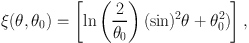
The momentum is introduced over a range of radii χ_w between four and eight grid cells from the source falling off as r⁻², and is modulated by a function of the polar angle θ and jet opening angle θ₀, ξ(θ,θ₀) given by

(35)

derived from Matzner and McKee, (1999). The connection with the simulation is made by inserting source terms into the density, momentum and energy equations.

An analogous model is implemented in flash by Federrath et al., (2014). Outflows are launched in spherical cones with opening angle θ₀ about the sink particle rotation axes, with θ₀ taken to be 30. The outflow mass inserted in a timestep Δ t is scaled to the sink particle accretion rate so that M_out = f_m Δ t, with f_m taken to be 0.3. 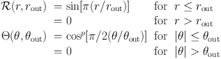The outflow mass is inserted uniformly inside the cones, but the outflow velocities are smoothed both with distance from the sink, and in an angular sense so that they drop to zero on the surfaces of the outflow cones, avoiding numerical instabilities. The chosen smoothing functions are as follows:

(36)

The outflow characteristic velocity is set to the Keplerian value appropriate for a star with the mass of the sink and a radius of 10 R_⊙. In order to produce a highly–collimated jet and a more extended ‘wind', the velocity profile is further modified to

(37)

The authors stress that they take particular care to correct the mass and momentum fluxes in the two outflow cones to ensure that global momentum is exactly conserved. They also transfer a fraction of the accreted angular momentum to the outflow.

4.4. Supernovae

Few authors have attempted to model the effects of supernovae on well–resolved individual clouds, probably because most GMC–scale simulations do not form any O–stars, or do not progress far enough in time for massive stars that do form to reach the ends of their lives. However, there are some notable exceptions.

Rogers and Pittard, (2013) extend their study of the impact of stellar winds on a turbulent molecular clump through the late and terminal stages of their three embedded O–stars. They follow the WR phase of each star and allow them to detonate as supernovae one after another by depositing 10⁵¹ erg and 10 M_⊙ of ejecta instantaneously.

Durier and Dalla Vecchia, 2012 set out to compare the relative efficacy of injecting supernova energy in thermal and kinetic form in SPH simulations, distributing energy amongst 32 particles nearest the explosion site. Both methods reproduced the Sedov solution well when global timesteps were employed, but poorly when individual particle timesteps were used. The two methods did agree in the case of individual particle timesteps if they were updated immediately after the energy release, and if the timesteps of neighbouring gas particles were forbidden from differing by more than a small factor (they suggest 4).

Using an SPH code, Walch and Naab, (2014) investigate the detonation of single explosions in clouds of mass 10⁵ M_⊙ and radius 16 pc, represented by 10⁶ particles. They take the ejecta mass to be 8 M_⊙ and represent the ejecta using particles of the same mass as those from which the cloud is built, resulting in there being 80 particles in the supernova remnant initially. The ejecta particles are randomly distributed in a 0.1pc sphere around the explosion source and given a radial velocity of 3 400 km s⁻¹, to give an explosion energy of 10⁵¹ erg (they also perform a simulation in which the ejecta particles are not given outward initial velocities, but instead carry the 10⁵¹ erg as thermal energy, finding similar results provided small timesteps are used for the ejecta particles and their neighbours). Thermodynamics are handled using a constant heating rate and a cooling rate constructed from the table in Plewa, (1995) and the analytical formula in Koyama and Inutsuka, (2000). Particle energies are integrated using substeps in cases when the cooling time becomes shorter than the particle's dynamical time. They are able to accurately reproduce the Sedov–Taylor phase of the remnant evolution, as well as the transition to the radiative pressure–driven snowplough stage.

4.5. Galactic–scale models

Simulations at the scale of a galactic spiral arm or disc can in general not model most of the feedback processes described above for want of resolution. An illustrative problem, for example, comes with the inclusion of supernovae in SPH simulations. On galactic timescales, a supernova is the instantaneous point release of a quantity of energy which must then be distributed in the gas near the explosion site. The mass resolution of an SPH simulation places a strict lower limit on the amount of material over which the explosion energy can be distributed, which in turn sets the temperature of the gas. If the mass is too high, the temperature can be much lower than that expected in a supernova remnant and is likely to lie in the thermally–unstable regime of the cooling curve. The energy will therefore be quickly radiated away. This issue has traditionally been circumvented by temporarily disabling cooling at supernova sites. Other problems arise from the tremendous dynamic ranges that need to be modelled. As discussed by Scannapieco et al., (2006), poor resolution of the interface between hot diffuse material and cold dense clouds, particularly in SPH, artificially raises the density and decreases the cooling time in the hot material.

Springel and Hernquist, (2003) implement a feedback model in the gadget SPH code designed to circumvent these problems. They implicitly assume that the gas consists of two phases – a hot rarefied phase and a cold dense phase. Mass exchange between the phases occurs via star formation, the evaporation of cold material to form hot material, and the cooling and condensation of hot material to form cool material.

Star formation occurs on a timescale t_*, and a fraction β of the stellar mass is immediately recycled into the hot phase via SNe, so that

(38)

The heating rate from supernovae, expressed in terms of the specific internal energy stored in the hot phase, is taken to be

(39)

with є_SN = 10⁴⁸ erg M_⊙⁻¹.

The cold phase is assumed to evaporate into the hot phase by a process similar to thermal conduction. The mass evaporated from the cold phase is taken to be proportional to the mass released from SNe, so that

(40)

The constant A is environmentally dependent, with its functional form taken to be A∝ρ^−4/5 and the normalisation treated as a parameter.

The cold phase is assumed to grow by thermal instability:

(41)

where Λ is a cooling function, and the thermal instability is only permitted to operate in gas whose density exceeds a threshold. Springel and Hernquist, (2003) showed that this model leads to self–regulated star formation, since star formation increases the evaporation rate of the cold clouds, which increases the density and cooling rate in the hot gas, thereby increasing the rate of formation of cold gas. A reasonable choice of A and the star formation timescale results in a star formation law resembling the SK law.

However, Springel and Hernquist, (2003) point out that the assumed tight coupling between the hot and cold phases does not permit them to model star–formation driven galactic winds. These are a vital component of galaxy formation, since they further suppress star formation by ejecting, or at least cycling, baryons into diffuse regions where star formation does not occur, and they also assist disc formation by expelling low–angular momentum material from haloes. They therefore additionally implement a parameterised wind model. The wind mass loss rate is taken to be proportional to the star formation rate, _w = η_* and the wind carries a fixed fraction of the total supernova energy output. Gas particles are entrained in the wind in a probabilistic fashion, so that in a timestep Δ t, the probability of entrainment is

(42)

where x is the mass fraction in the cold phase. In order to prevent wind particles being trapped inside thick discs, their hydrodynamic interaction with other particles is disabled for a period of 50 Myr.

Scannapieco et al., (2006) improve upon this model with a more sophisticated treatment of SNe. Star particles are assigned two smoothing lengths, enclosing equal masses of the hot and cold gaseous phases only. Supernova energy is divided between the hot and cold phases, weighted by the corresponding smoothing kernel. The fraction є_h assigned to the hot phase is injected as thermal energy. A second fraction є_r is assumed to be radiated away by the cold phase and lost. The remainder, 1−є_h−є_r is injected into the cold phase. Cold particles accumulate supernova energy until their thermodynamic properties are similar to their hot neighbours', at which point they are ‘promoted' to the hot phase. є_h and є_r are then treated as free parameters and adjusted to obtain the desired ISM properties.

A novel approach to the inclusion of supernova feedback is presented by Teyssier et al., (2013), who introduce a new variable є_turb which represents the density of non–thermal energy and whose evolution is followed via

(43)

where _inj = _* η_SNє_SN is the feedback energy injection term composed of the star formation rate, an efficiency factor and the energy per supernova, and t_diss is a dissipation timescale, which they set to 10 Myr, comparable to the typical GMC lifetime (although they discuss several other possibilities). Feedback is connected to the hydrodynamics by defining є_turb = ρσ_turb² / 2 and modifying the total pressure to include thermal and turbulent terms, so that P_tot = P_therm + ρσ_turb². A similar scheme has been explored by Agertz et al., (2013).

Other authors attempt to model supernovae in a more explicit manner in similar fashion to simulations at GMC scales. In flash Gatto et al., (2015) inject 10⁵¹ erg of supernova energy into a region containing 10³ M_⊙ of gas or eight grid cells across, whichever is larger. If thermalisation of this energy would result in temperatures above 10⁶ K, the energy is inserted in thermal form. However, at higher densities and masses, the overcooling problem would be encountered, essentially because the Sedov–Taylor phase of the remnant cannot be resolved. Gatto et al., (2015) get around this problem by computing, given the actual density in the injection region, the expected bubble radius and momentum at the end of the Sedov–Taylor phase and injecting this momentum into the cells instead, while also heating them to 10⁴ K.

Hopkins et al., (2011) and Hopkins et al., (2012) point out that, on galactic scales, most of the gas is so dense that it cools efficiently – only ∼ 10 percent of the total ISM pressure comes from the hot ISM. In denser regions, momentum dominates and radiation pressure, stellar winds and supernovae are all comparable when averaged over galactic dynamical timescales. Ostriker and Shetty, (2011) make a similar point. Hopkins et al., (2011) identify star–forming clumps around the densest gas particles and compute the stellar bolometric luminosity within the clump using starburst–99 (Leitherer et al., 1999) models and a Kroupa IMF. They assume that the momentum is distributed equally amongst all gas particles within a clump and for a given particle j in a clump, the imparted momentum flux is then

(44)

with L_j = (M_gas,j / M_gas,clump) L_clump. The first factor in the brackets represents momentum deposited in the gas by dust absorption of the optical and UV photons from the massive stars. The dust reradiates in the infrared and the second term allows for absorption of this radiation. τ_IR is the optical depth across the clump, equivalent to a trapping factor, and η_p ≈ 1 is a parameter which can be adjusted to allow for other sources of momentum, e.g. jets, winds and SNe (η_p > 1), or for photon leakage (η_p < 1). A similar model is presented in Agertz et al., (2013) but their cosmological–scale simulations do not have the resolution to estimate the infrared optical depths, so these are estimated from subgrid models.

As well as the momentum imparted by winds and SNe, they include the thermal energy released by the associated shocks, again tabulated from starburst–99 models, and including AGB winds as well as main–sequence and WR winds. This energy is deposited over the SPH smoothing kernels of the dense gas particles defining the star–forming clump centres. Photoionisation heating is implemented by finding particles within the Strömgren spheres centred on the clumps and heating the gas inside to 10⁴ K (or preventing it from cooling below this temperature).

Hopkins et al., (2011) and Hopkins et al., (2012) also allow for the fact that feedback partially or completely disrupts GMCs, so that substantial quantities of the IR and UV photons released inside them escape and are only absorbed at larger distances. Hopkins et al., (2012) allow the energy to spread over the larger of the local gas smoothing length or the local gravitational softening length.

Ceverino et al., (2014) discuss a similar scheme for including radiation pressure from ionising photons where the gas is assumed to be locally optically thin. The radiation pressure is taken to be one third the radiation energy density, P_rad = 4π I / (3c) and isotropic. The intensity I is computed using starburst–99 (Leitherer et al., 1999) as a function of the stellar mass, spread over a reference area A, so that I = Γ m_* / A and P_rad = Γ m_* / (R² c), R being set to half a grid cell size for cells containing stellar mass, and one grid cell size for neighbours of such cells. If the gas density in the cell exceeds 300 cm⁻³, the radiation pressure is boosted by a factor of (1 + τ), where τ = n_cell / 300 cm⁻³ to account approximately for the trapping of infrared radiation in optically–thick gas. Using cloudy (Ferland et al., 1998) models, they also account of the change in the local heating and cooling rates resulting from irradiation by stellar populations of different ages with different SEDs.

Roskar et al., (2014) model radiation fields at galactic scales using an escape probability formalism and splitting the radiation field into UV and IR components. The energy absorbed from the UV field is taken to be E_UV = E_rad[1 − exp(−κ_UV ρ_dustΔ x)], where E_rad = 10⁵² erg M_⊙⁻¹ is the total specific energy released by a 10 M_⊙ star. It is then assumed that the absorbed UV radiation is reemitted in the infrared, so that E_IR = E_UV[1 − exp(−κ_IR ρ_dust Δx)]. The dust opacity is treated as a free parameter. This energy is then added to the supernova feedback energy, and effectively deposited as momentum.