


2.1. Dynamical Parameters Representing the Galaxy
In this review, we use either the traditional galactic constants of (R0, V0) = (8.0 kpc, 200 km s−1), or the recently determined values, (R0, V0) = (8.0 kpc, 238 km s−1) from observations using VERA (VLBI Experiment for Radio Astrometry) (Honma et al. 2012; 2015). Here, R0 is the distance of the Sun from the Galactic Center and V0 is the circular velocity of the Local Standard of Rest (LSR) at the Sun (see Fich and Tremaine 1991 for review).
An approximate estimation of the mass inside the solar circle can be obtained for a set of parameters of R0 = 8 kpc and V0 = 200 to 238 km s−1, assuming spherical distribution of mass, as
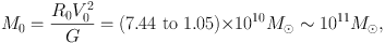 |
(1) |
with G being the gravitational constant, and the Solar rotation velocity V0 being related to R0 as V0 = (A−B)R0, A and B are the Oort's constants, which are determined by measuring radial velocity and proper motion of a nearby star. See Kerr and Lynden-Bell (1986) for a review about the Oort constants, and tables 1 and 2 for recent values.
| Authors (year) | A km s−1 kpc−1 | B km s−1 kpc−1 |
| IAU recommended values (1982) | 14.4 ± 1.2 | −12.0 ± 2.8 |
| HIPPARCOS (Feast and Whitelock 1997) | 14.8 ± 0.8 | −12.0 ± 0.6 |
| Cepheids (Dehnen and Binney 1998) | 14.5 ± 1.5 | −12.5 ± 2 |
| Dwarfs, infrared photometry (Mignard 2000) | 11.0 ± 1.0 | −13.2 ± 0.5 |
| —- Distant giants | 14.5 ± 1.0 | −11.5 ± 0.5 |
| Stellar parallax (Olling and Dehnen 2003) | ≃ 16 | ≃ −17 |
| Authors (year) | R0 kpc | V0 km s−1 |
| IAU recommended (1982) | 8.2 | 220 |
| Review before 1993 (Reid 1993) | 8.0 ± 0.5 | |
| Olling and Dehnen 1999 | 7.1 ± 0.4 | 184 ± 8 |
| VLBI Sgr A* (Ghez et al. 2008) | 8.4 ± 0.4 | |
| ibid (Gillessen et al. 2009) | 8.33 ± 0.35 | |
| Maser astrometry (Reid et al. 2009) | 8.4 ± 0.6 | 254 ± 16 |
| Cepheids (Matsunaga et al. 2009) | 8.24 ± 0.42 | |
| VERA (Honma et al. 2012, 2015) | 8.05 ± 0.45 | 238 ± 14 |
By the definition of rotation curve, we assume that the motion of gas and stars in the Galaxy is circular. This assumption put significant limitation on the obtained results. In fact, the galactic motion is superposed by non-circular streams such as a flow due to a bar, spiral arms, and expanding rings. The dynamical parameters of the Galaxy to be determined from observations, therefore, include those caused both by axisymmetric and non-axisymmetric structures. In table 3 we list the representative parameters and analysis methods (Sofue 2013b).
| Subject | Component | No. of Parameters | |
| I. Axisymm. | Black hole | (1) Mass | |
| structure | Bulge(s)‡ | (2) Mass | |
| (RC) | (3) Radius | ||
| (4) Profile (function) | |||
| Disk | (5) Mass | ||
| (6) Radius | |||
| (7) Profile (function) | |||
| Dark halo | (8) Mass | ||
| (9) Scale radius | |||
| (10) Profile (function) | |||
| II. Non-axisymm. | Bar(s) | (11) Mass | |
| structure | (12) Maj. axis length | ||
| (out of RC) | (13) Min. axis length | ||
| (14) z-axis length | |||
| (15) Maj. axis profile | |||
| (16) Min. axis profile | |||
| (17) z-axis profile | |||
| (18) Position angle | |||
| (19) Pattern speed Ωp | |||
| Arms | (20) Density amplitude | ||
| (21) Velocity amplitude | |||
| (22) Pitch angle | |||
| (23) Position angle | |||
| (24) Pattern speed Ωp | |||
| III. Radial flow | Rings | (25) Mass | |
| (out of RC) | (26) Velocity | ||
| (27) Radius | |||
| † In the present paper we review on subject I. | |||
| ‡ The bulge and bar may be multiple, increasing the number of parameters. | |||
In the present paper, we review the methods to obtain parameters (1) to (10) in the table, which define the axisymmetric structure of the Galaxy as the first approximation to the fundamental galactic structure. Non-circular motions caused by a bar and spiral arms are beyond the scope of this review, which are reviewed in the literature (e.g., Binney et al. 1991; Jenkins and Binney 1994; Athanassoula 1992; Burton and Liszt 1993).
2.2. Progress in the Galactic Rotation Curve
Figure 1 shows the progress in the determination of rotation curve of the Milky Way Galaxy. Before and till the 1970's the inner rotation curve of the Milky Way has been extensively measured by the terminal-velocity method applied to radio line observations such as the HI line (Burton and Gordon 1978; Clemens 1985; Fich et al. 1989).
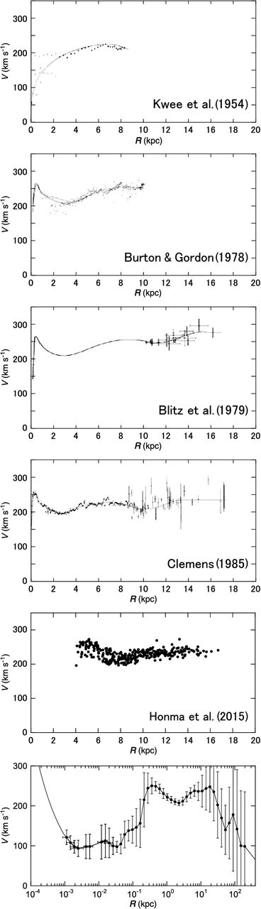 |
Figure 1. Half a century progress in rotation curve (RC) determination of the Milky Way. Top to bottom: 1950's (Kwee et al. 1954); 1970's CO and HI (Burton and Gordon 1978; Blitz et al 1979); 1980's Composite of CO, HI and optical (Clemens 1985); 2001's most accurate trigonometric RC by maser sources with VERA (Honma et al. 2015); and a semi-logarithmic grand RC from the Galactic Center, linked to the massive black hole, to half a way to M31 (Sofue 2015a). |
In 1980 to 1990's, outer rotation velocities of stellar objects (OB stars) were measured by combining optical distances and CO-line velocities of associating molecular clouds (Blitz et al. 1982; Demers and Battinelli 2007). The HI thickness method was also useful to measure rotation of the entire disk (Merrifield 1992; Honma and Sofue 1997).
In 1990 to 2000's, VLBI measurements of parallax and proper motions of maser sources and Mira variable stars have provided with advanced rotation velocities with high accuracy (Honma et al. 2007). It was also recent that proper motions of a considerable number of stars were used for rotation curve measurement (Lopez-Corredoira et al. 2014).
The most powerful tool to date to measure the rotation of the Milky Way up to R ∼ 20 kpc is the VERA, with which trigonometric determination of both the 3D positions and velocities are done simultaneously for individual maser sources (Honma et al. 2007; 2012; 2015; Sakai et al 2015; Nakanishi et al. 2015).
Since 1990's, with the kinematics of interstellar gas and infrared stars in the vicinity of the nucleus of our Galaxy, Sgr A*, the existence of the massive black hole has been revealed. The black hole mass on the order of ∼ 4 × 10⁶ M⊙ was measured by proper-motion measurements of infrared sources around the nucleus (Genzel et al. 1994; Ghez et al. 1998; Lindqvist et al. 1992; Gillessen et al. 2009).
For the total mass of the Galaxy including the extended dark halo, analyses of the outermost rotation curve and motions of satellite galaxies orbiting the Galaxy have been obtained in detail. The total mass of the Galaxy including the dark halo up to ∼ 150 kpc has been estimated to be ∼ 3 × 10¹¹M⊙. (Sofue 2015b).
| Authors (year) | Radii | Method | Remark |
| Burton and Gordon (1978) | 0 - 8 kpc | HI tangent | RC |
| Blitz et al. (1979) | 8 - 18 kpc | OB-CO association | RC |
| Clemens (1985) | 0 -18 kpc | CO/compil. | RC |
| Dehnen and Binney (1998) | 8 - 20 | compil. + model | RC/Gal. Const. |
| Genzel et al. (1994–), Ghez et al. (1998–), et al. | 0–0.1 pc | IR spectroscopy | Orbits, velo. dispersion |
| Battinelli, et al. (2013) | 9 - 24 kpc | C stars | RC |
| Bhattacharjee et al.(2014) | 0 - 200 kpc | Non-disk objects | RC/model fit |
| Lopez-Corredoira (2014) | 5 - 16 kpc | Red-clump giants µ | RC |
| Bobylev (2013); — & Bajkova (2015) | 5 - 12 kpc | Masers/OB stars | RC/Gal. const. |
| Honma et al. (2012, 2013, 2015) | 3 - 20 kpc | Masers, VLBI | RC/Gal. const. |
| Sofue et al. (2009); Sofue (2013b, 2015a) | 0 - 300 kpc | CO/HI/opt/compil. | RC/model fit |
2.3. Methods to Determine the Galactic Rotation Curve
The radial velocity, vr, and perpendicular velocity to the line of sight, vp, of an object at a distance r orbiting around the Galactic Center are related to the circular orbital rotation velocity V as
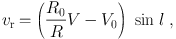 |
(2) |
and
 |
(3) |
where
 |
(4) |
Here µ is the proper motion, and R is the galacto-centric distance related to r and galactic longitude l by
 |
(5) |
or
 |
(6) |
2.3.1. Terminal-velocity method inside the solar circle
Inside the solar circle, the galactic disk has tangential points, at which the rotation velocity is parallel to the line of sight. Figure 2 shows the tangent velocities measured for the 1st quadrant of the galactic disk (e.g., Burton and Gordon 1978).
 |
Figure 2. CO and HI line tangent velocities for the inner rotation curve (Burton and Gordon 1978) |
Maximum radial velocities vr max (terminal or the tangent-point velocity) are measured by the edges of spectral profiles in the HI and CO line emissions at 0 < l < 90∘ and 270 < l < 360∘. The rotation velocity V(R) is calculated using this velocity as
 |
(7) |
and the galacto-centric distance is given by
 |
(8) |
The method to calculate the rotation velocity using the radial velocity is applied to various objects, where
 |
(9) |
In this method, the distance r has to be measured independently of other methods such as trigonometric and/or spectroscopic measurements. Often used objects are OB stars or association. The distances of OB stars are measured from their distance modulus, and the distance is assumed to be the same as that of its associated molecular cloud or HII region whose radial velocity is observed by molecular/recombination line measurements. However, errors in the photometric distances are usually large, resulting in large errors and scatter in the outer rotation curve determinations.
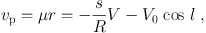
The rotation velocity can be also measured by using proper motion µ as
 |
(10) |
VLBI techniques have made it possible to employ this method, where the distance r, proper motion vp (= r µ), and radial velocity vr are observed at the same time. Applying this technique to a number of maser sources, the outer rotation curve has been determined with high accuracy (Honma et al. 2012, 2015; Sakai et al. 2012, 2015; Nakanishi et al. 2015) (figure 1).
Proper motions of a large number of stars from HYPPARCOS observations combined with the 2MASS photometric data have recently been analyzed for galactic kinematics (Roeser et al 2010; Lopez-Corredoira 2014). Proper motions were obtained from PPMXS catalogue from HYPPARCOS observations, and the distances were determined from K and J band photometry using 2MASS star catalogue correcting for the interstellar extinction. The RCG stars were used for their assumed constant absolute magnitudes.
2.3.4. Trigonometric method using velocity vectors with VLBI
The ultimate method to investigate the Milky Way's rotation, without being bothered by various assumptions such as the circular rotation and/or a priori given solar constants, is the VLBI method, by which three-dimensional (3D) positions and motions of individual maser sources are measured simultaneously.
The VERA observations have most successfully obtained rotation velocities for several hundred galactic maser sources within ∼ 10 kpc from the Sun. This project has introduced a new era in Galactic astronomy, providing us with the most precise solar constants ever obtained (Honma et al. 2007; 2012; 2015; Sakai et al 2015; Nakanishi et al. 2015).
When the three independent quantities of vr, µ, and r are known or have been observed simultaneously, the three-dimensional velocity vector can be determined uniquely without making any assumptions such as a circular orbit. The absolute value of the velocity vector is given by
 |
(11) |
where
 |
(12) |
and
 |
(13) |
In the current methods distances of individual objects are measured independently of radial velocities or proper motions. However, distances of diffuse and/or extended interstellar gases are not measurable. The HI-disk thickness method has been developed to avoid this inconvenience (Merrifield 1992; Honma and Sofue 1997), where annulus-averaged rotation velocities are determined in the entire disk. In the method, the angular thickness Δb of the HI disk is measured along an annulus ring of radius R, which is related to R and l by
 |
(14) |
The longitudinal variation of Δb is uniquely related to the galacto-centric distance R, and is as a function of V(R). Since this method measures the averaged kinematics of the Galaxy, it represents a more global rotation curve than those based on the previous described methods.
2.4. Rotation in the Galactic Center
For its vicinity the Galactic Center rotation has been studied in most detail among the spiral galaxies, particularly in the nuclear region around Sgr A* nesting the super massive black hole.
Extensive CO-line observations of the Galactic Center have provided us with high quality and high-resolution longitude-velocity (LV) diagrams in the Galactic Center (e.g., Dame et al. 2001; Oka eta l. 1998). Figure 3 shows the rotation curve in the central ∼ 100 pc as obtained by applying the terminal-velocity method to these LV diagrams (Sofue 2013b).
 |
Figure 3. Rotation velocities in the Galactic Center obtained by terminal-velocity method using PV diagrams (grey dots: measured values; circles: running averaged values) (Sofue 2013). |
Further inside ∼ 0.1 pc of the Galactic Center, infrared proper-motion measurements of circum-nuclear giant stars have shown that the stars are moving around Sgr A* in closed elliptical orbits. Analyses of the orbits showed high velocities that increase toward the nucleus, giving firm evidence for a massive black hole located at the same position as Sgr A* of ∼ 4 million solar masses (see section 4.2.2).
2.5. Logarithmic Rotation Curve: From Black Hole to Dark Halo
A rotation curve covering wider regions of the Galaxy has been obtained by compiling the existing data by re-scaling the distances and velocities to the common galactic constants (R0, V0) = (8.0 kpc, 200 km s−1) (Sofue et al. 2009). Rotation velocities in the outermost Galaxy and beyond the disk were estimated by analyzing radial velocities of globular clusters and satellite galaxies (Sofue 2013b).
Figure 4 shows a logarithmic rotation curve of the entire Milky Way. The enlarged scale toward the center is useful to analyze the nuclear dynamics. The curve is drawn to connect the central rotation curve smoothly to the Keplerian motion representing the central massive black hole of mass 3.6 × 10⁶ M⊙ (Ghez et al. 2005; Gillesen et al. 2009). This figure shows the continuous variation of rotation velocity from the Galactic Center to the dark halo.
 |
Figure 4. Logarithmic rotation curve of the Galaxy for V0 = 238 km s−1 and deconvolution into a central black hole, two exponential-spherical bulges, exponential flat disk, and NFW dark halo by the least χ2 fitting shown by thin lines. A classical de Vaucouleurs bulge shown by the dashed line is significantly displaced from the observation. |
Detailed analyses of the rotation curve and deconvolution into mass components will be described in chapter 4.
2.6. Uncertainty and Limitation of Rotation Curve Analyses
The accuracy of the obtained rotation curve of the Milky Way is determined not only by the measurement errors, but also by the employed methods and the location of the observed objects in the Galactic disk (Sofue 2011).
The most common method to calculate rotation velocity V using the radial velocity vr and distance r yields
 |
(15) |
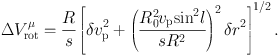
The error of the derived velocity is given by
 |
(16) |
where
 |
(17) |
Remembering equations (5) and (9) we obtain
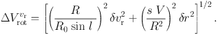 |
(18) |
The rotation velocity using the proper motion vp is given by
 |
(19) |
Knowing R2 − s2 = R02 sin2 l, we have the errors in this quantity as
 |
(20) |
In figure 5 we present examples of the accuracy diagram of the radial velocity method for a set of measurement errors, δ vr = 1 km s−1 and δr / r = 0.02 , or 2%. It is readily seen that the accuracy is highest along the tangent point circle (white regions), proving that tangent-point circle is a special region for accurate rotation curve determination. On the contrary, it yields the largest error near the singularity line running across the Sun and the Galactic Center, where the circular rotation is perpendicular to the line-of-sight.
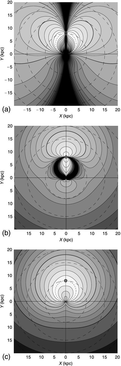 |
Figure 5. (a) Accuracy diagrams ΔVrotvr(X, Y) for δvr = 1 km s−1 and 2% distance error, (b) ΔVrotµ(X, Y) for δµ = 0.2 mas y−1, and (c) ΔVrotvec(X, Y) for δvp /r = 1 km s−1 kpc−1 corresponding to δµ = 0.21 mas y−1, δvr = 1 km s−1 , and 2% distance error (Sofue 2011). |
In figure 5(b) we show an accuracy diagram of the proper-motion method for δvp / r = 1 km s−1 kpc−1, or δµ = 0.21 mas y−1, and δr / r = 0.02. Contrary to the radial velocity method, the error becomes smallest along the Sun-GC line, but it is largest near the tangent point circle, where equation 20 diverges. Thus, the tangent-point circle is a singular region in this method. This behavior is just in opposite sense to the case for the radial-velocity method, and the radial-velocity and the proper-motion methods are complimentary to each other.
Figure 5(c) shows the same, but for errors in velocity vector method using the 3D trigonometric measurement. This method yields much milder error variations in the entire Galaxy, showing no singular regions.
The accuracy diagram, ΔVrotvr(X, Y), demonstrates the reason why the rotation curve is nicely determined along the tangent-point circle, which is a special region yielding the highest accuracy determination of rotation velocity. The diagram also suggests that the butterfly areas at l ∼ 100−135∘ and l ∼ 225−280∘ are suitable regions for outer rotation curve work using the radial-velocity method.
In the proper motion method, the most accurate measurement is obtained along the Sun-Galactic Center line, as was indeed realized by Honma et al. (2007). It must be also emphasized that the minimum error area is widely spread over l ∼ 120 − 250∘ in the anti-center region, as well as in the central region inside the tangent-point circle. On the other hand, the largest error occurs along the tangent-point circle, which is the singularity region in this method.
2.7. Radial-Velocity and Proper-Motion Fields
If the rotation curve is determined, we are able to measure kinematical distances of any objects in the galactic disk by applying the velocity-space transformation, assuming circular rotation of the objects (Oort et al. 1958; Nakanishi and Sofue 2003, 2006, 2015). The kinematical distance is obtained either from radial velocity or from proper motion using equations (2) and (3), and the velocities can be represented as a map on the galactic plane, as shown in figure 6.
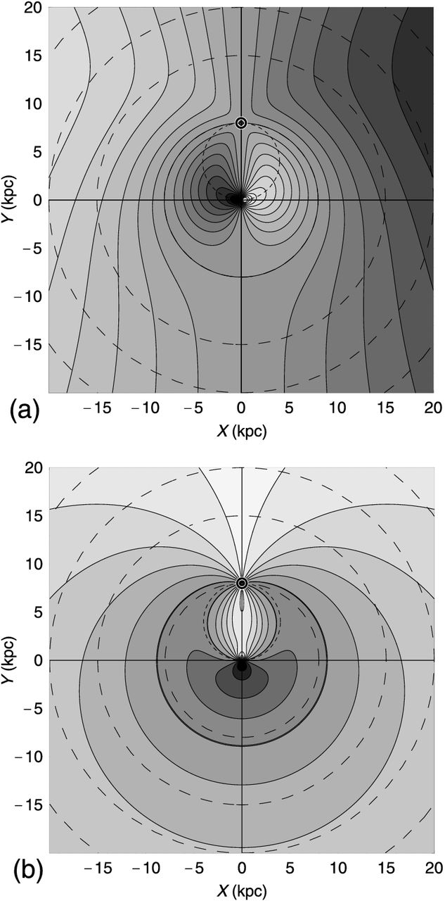 |
Figure 6. (a) Radial velocity field vr(X, Y) with contour increment 20 km s−1 , and (b) proper motion field µ(X, Y) with contour increment 1 mas y−1. The circle near the solar orbit is for 5 mas y−1. |
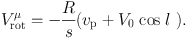
It may be worth to mention that the solar circle is a special ring, where the radial velocity is zero, vr = 0, whereas the proper motion µ has a constant value with
 |
(21) |
which yields µ⊙ = −5.26 mas y−1 for R0 = 8 kpc and V0 = 200 km s−1 .
VLBI trigonometric measurements have made it possible to apply this method to determine kinematical distance rµ. However, the radial-velocity field is currently used more commonly to map the distributions of stars and interstellar gas in the galactic plane because of its convenience.
2.8. Velocity-to-Space Transformation
If a rotation curve V(R) is obtained or assumed, the radial velocity vr of an object in the galactic disk is uniquely calculated by equation (2). Figure 6 shows a thus calculated distribution of the radial velocity, or the velocity field. Equation (2) includes the distance and longitude. Therefore, the equation can be solved inversely to determine the position of an object using its radial velocity. This procedure is called the velocity-to-space (VTS) transformation.
By this method, the position of an object outside the solar circle is uniquely determined, but it has two-fold solutions for objects inside the solar circle. In order to solve this two-folding distance problem, further information such as apparent sizes of individual clouds and/or disk thickness is employed.
Applying the VTS transformation, galactic maps of HI and H2 gases are obtained as follows. Column densities of HI and H2 gases are related to the HI and CO line intensities as
 |
(22) |
and
 |
(23) |
where THI and TCO are the HI and CO line brightness temperatures, and Ci are the conversion factors, and CHI = 1.82 × 10¹⁸ [H cm−2] and CH2 ∼ 2 × 10²⁰ f(R, Z) [H2 cm−2] are the conversion factors, and f is a correction factor depending on R (e.g. Arimoto et al. 1996).
Volume density of the gas corresponding to radial velocity vr is obtained by
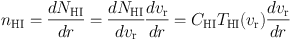 |
(24) |
and
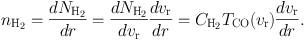 |
(25) |
These formulae enables us to create a face-on view of the ISM in the Galaxy, where the three-dimensional distribution of the volume densities of the HI and H2 gases can be mapped. Fig. 7 shows the thus obtained face-on view of the Galactic disk (Nakanishi and Sofue 2003, 2006, 2015).
 |
Figure 7. [Top] 2D HI map of the Galaxy, showing the distribution of volume density of the HI gas in the galactic plane on the assumption of circular rotation of the disk (Oort and Kerr 1958). [Middle] Surface densities of HI (contours) and H2 (grey scale) gases obtained by integrating the 3D maps in the Z direction (Nakanishi and Sofue 2016). [Bottom] HI and H2 cross-section map of the Galaxy in the (X, Z) plane across the Galactic Center. Shown here are the volume densities HI (extended thick disk in gray scale) and H2 (thin disk by contours) (Sofue and Nakanishi 2016). Note, the Z axis is enlarged by a factor of 4. |