


In this section we move away from the study of the all-sky average of the DGRB, focusing on what can be learnt from its spatial fluctuations. Note that, following the procedure outlined in Sec. 2,1 and used in Ref. [9], the DGRB should be isotropic by construction. Yet, the template fitting is not sensitive to moderate small-scale anisotropies in the emission. 29 A well-established strategy to quantify the amount of spatial fluctuations is the anisotropy APS. Traditionally employed for the study of the CMB [254], the technique consists in decomposing a 2-dimensional map I(n) in spherical harmonics Yℓ,m(n): I(n) = ∑ℓ,m aℓ,m Yℓ,m(n). The APS Cℓ is, then, computed as follows:
 |
(24) |
A measurement of the APS of the DGRB provides information on its composition that is complementary to the study of its intensity energy spectrum. In Sec. 3.1 we summarize the measurement of the DGRB anisotropies performed by the Fermi LAT in Ref. [66]. Then, in Sec. 3.2, we describe how such a measurement can be used to constrain the DGRB contributors. 30
3.1. The Fermi LAT measurement of gamma-ray anisotropies
The measurement performed by the Fermi LAT Collaboration in Ref. [66] is currently the only observational data available on the APS of the DGRB. 22 months of data are analyzed between 1 and 50 GeV, divided in 4 energy bins. Gamma rays are binned into a HEALPix map 31 [402] with Nside = 512. The count maps are divided by the exposure of the instrument in order to obtain gamma-ray intensity maps. This is required in order to eliminate any spurious spatial fluctuations due to the non-uniform exposure of Fermi LAT.
Two definitions of the APS are used in Ref. [66]. The so-called intensity APS Cℓ is obtained from Eq. (24), while the fluctuation APS Cℓfluct comes from the decomposition of the relative fluctuations I(n) / ⟨ I ⟩, where ⟨ I ⟩ is the all-sky average intensity. The two definitions are related by Cℓfluct = Cℓ / ⟨ I ⟩2. Note that the fluctuation APS is a dimensionless quantity, while Cℓ inherits the units of the intensity map (squared).
Contrary to what is done in Ref. [9] (see Sec. 2.1), no template fitting is employed in Ref. [66] to isolate the DGRB. Nevertheless, a mask is applied, screening the regions in the sky where the emission is dominated by the diffuse Galactic foreground or by the resolved point sources. The mask covers the strip with |b| < 30° around the Galactic plane and a 2°-radius circle around each source in the 1FGL catalog. The contamination of the Galactic foreground is not completely removed by the use of the mask, but the residual Galactic emission only induces large-scale features that contribute to the APS at small multipoles. That is why only multipoles larger than 105 are considered in Ref. [66].
The mask may alter the shape and normalization of the APS. Following Ref. [403], the APS is corrected for the effect of the mask simply by dividing Cℓ by the fraction of unmasked sky, fsky. Therefore, the APS estimator considered in Ref. [66] is
 |
(25) |
where Cℓraw is the intensity APS computed directly from the masked intensity maps. CN is the so-called photon noise, i.e. CN = ⟨ I ⟩2 4 π fsky / Nγ, where Nγ is the total number of events detected outside the mask. Finally, the factor Wℓbeam corrects for the smearing induced by the Point Spread Function (PSF) of the telescope (see Ref. [66] for a definition of Wℓbeam). The effect of the PSF becomes too extreme for angular scales beyond ℓ = 504 so that, in Ref. [66], no data are considered for multipoles larger than ℓ = 504.
Fig. 13 shows the APS for gamma rays between 1.99 and 5.0 GeV. The data points show the weighted average of the APS inside bins in multipoles with Δℓ = 50. The purple crosses correspond to the APS estimator Cℓ of Eq. (25) derived from the intensity maps. On the other hand, the empty red boxes indicate the APS measured from the residual maps obtained after the subtraction of a model for the diffuse Galactic foreground. The error bars are computed following Ref. [404]. 32
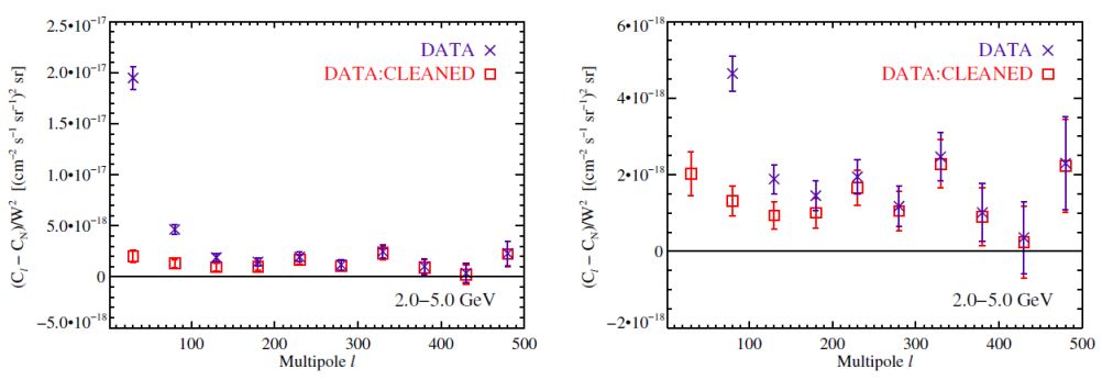 |
Figure 13. Intensity APS of the data before (purple crosses) and after (red boxes) the removal of the diffuse Galactic foreground. The signal region is defined between ℓ=155 and 504. The large increase in the intensity APS with no foreground subtraction (purple crosses) at ℓ<155 is likely attributable to contaminations from the Galactic foreground emission. The right panel is an expanded version of the left panel and it focuses on the high-multiple angular power. Taken from Ref. [66]. |
The measured APS is different from zero in the signal region, i.e. 155 ≤ ℓ ≤ 504. The (unbinned) APS is fitted with a power law (ℓ/155)n in order to determine any dependence of the APS on ℓ. It is found that the n = 0 case is compatible with the best fit at 95% confidence level for all energy bins. This means that the measured APS is compatible with being Poissonian, i.e. independent of ℓ. The significance of the detection is 6.5 (7.2) between 1.04 and 1.99 GeV (between 1.99 and 5.0 GeV), while it decreases to 4.1 and 2.7 in the two remaining bins at higher energies.
The fluctuation APS of a population of sources depends on the energy only if their spatial clustering is itself energy-dependent or if they are characterized by significantly different energy spectra. On the other hand, their intensity APS scales with the energy as ⟨ I ⟩2. When computing the APS of an emission that is the sum of different components (as in the case of the DGRB), it may be interesting to study how the APS of the total emission Cℓtotal depends on the spectra of the individual components Cℓi. By construction, the intensity APS is an addictive quantity: 33
 |
(26) |
while the fluctuation APS follows the following summation rule:
 |
(27) |
where fi is the fraction of the emission associated with the i-th contribution, with respect to the total, i.e. fi = ⟨ Ii ⟩ / ⟨ Itotal⟩.
Assuming that the components have an energy-independent Cℓfluct,i, any energy dependence in Cℓfluct,total must arise from the fi-factors in Eq. (27). Indeed, Ref. [359] proves that detecting an energy modulation in the fluctuation APS of the DGRB may indicate that the emission is the sum of more components (see also Refs. [407, 408]). In that case, the behavior of the intensity APS as a function of energy would follow the energy spectrum of the dominant component. Thus, studying if (and how) fluctuation and intensity APS depend on the energy may be crucial to unravel the composition of the DGRB.
Fig. 14 shows the Poissonian Cp measured in Ref. [66] in the 4 energy bins 34. The left panel proves that the fluctuation APS does not depend on the energy. 35 On the other hand, the right panel shows that Cp decreases with energy as Cp ∝ E−(4.79 ± 0.13). This result suggests that the Fermi LAT APS is produced by one single population of unclustered sources with an energy spectrum proportional to ∝ E−2.40. In the next section we will see that unresolved blazars fits this description.
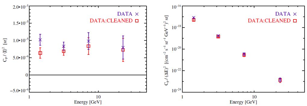 |
Figure 14. Anisotropy energy spectra of the data (purple crosses) and of the Galactic-foreground-cleaned data (red boxes). Left: Fluctuation anisotropy energy spectrum. Right: Differential intensity anisotropy energy spectrum. Taken from Ref. [66]. |
After the publication of the Fermi LAT APS measurement, Ref. [409] pointed out that the Fermi LAT Collaboration used 22 months of data to measure the APS, but masked only the contribution of the point-like sources in the 1FGL (relative to an exposure of only 11 months). Thus, the emission considered in Ref. [66] will probably be contaminated by the contribution of sources that, being not bright enough to be included in the 1FGL, could have been detected in the larger dataset of Ref. [66].
3.2. Deducing the nature of the Diffuse Gamma-Ray Background from its anisotropies
We start this section by summarizing the technique used to estimate the APS of a generic class of sources. The discussion will, then, focus on the gamma-ray emitters considered in Secs. 2.2 and 2.3. We will finally show how the comparison of the model predictions to the APS signal detected by the Fermi LAT in Ref. [66] can be used to constrain the contribution of different populations to the DGRB.
As done at the beginning of Sec. 2.2, the formalism proposed here assumes that the sources are characterized by a generic parameter Y. However, Eq. (1) only determines the all-sky average gamma-ray emission associated with population X, referred to here as ⟨ IX ⟩ to underline that it is obtained by integrating over all the possible pointings in the sky. The emission IX(n) from direction n can be written as follows [51, 107, 406]:
 |
(28) |
where χ = χ(z) is the comoving distance relative to redshift z. WX(χ) is the so-called window function and it gathers all the quantities that, in the definition of IX(n), do not depend on the direction of observation. In particular, WX(χ) may depend on the energy at which IX is computed. The factor gX(χ, n) is called the “source field” and it describes how IX changes from point to point in the sky. It encodes the dependence on the abundance and distribution of the sources. The averaged source field, ⟨ gX ⟩, can be used to write ⟨ IX ⟩ as ∫dχ ⟨ gX(χ) ⟩ WX(χ). The average source field depends only on the abundance of sources and it can be written as: 36
 |
(29) |
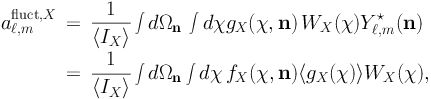
The aℓ,mfluct,X coefficients of the fluctuation APS of population X can be computed decomposing the relative intensity fluctuations IX(n) / ⟨ IX ⟩ in spherical harmonics, as follows:
 |
(30) |
where dΩn indicates the angular integration. Now, from Eq. (28)
 |
(31) |
where fX(χ,n) = gX(χ,n) / ⟨ gX ⟩. The fluctuation APS is obtained from the average of |aℓ,mfluct,X|2 with the same multipole ℓ, see Eq. (24). It can be shown [51, 406] that it is equivalent to:
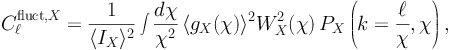 |
(32) |
where PX(k, χ) is the 3-dimensional power spectrum of the field fX(χ, n):
 |
(33) |
and  X
indicates the Fourier transform of the field
fX. Eq. (32) makes use of the so-called Limber
approximation
[410,
411],
valid for ℓ ≫ 1. This is indeed the regime of interest
here since the Fermi LAT APS measurement is robust only for
ℓ ≥ 155.
X
indicates the Fourier transform of the field
fX. Eq. (32) makes use of the so-called Limber
approximation
[410,
411],
valid for ℓ ≫ 1. This is indeed the regime of interest
here since the Fermi LAT APS measurement is robust only for
ℓ ≥ 155.
The hypothesis of working with a collection of unresolved sources allows the decomposition of the 3-dimensional power spectrum PX into a 1-halo term and a 2-halo term, P1h and P2h, respectively. This helps in the interpretation of PX and it allows to express it easily in the context of the Halo Model. The 1-halo term accounts for the correlation between two points located within the same source, while P2h describes the correlation between points that reside in different objects and, thus, it depends on the spatial clustering of the sources. Within the Halo Model formalism, 1-halo and 2-halo terms can be written, respectively, as follows [51, 52, 406]:
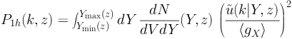 |
(34) |
and
 |
(35) |
The factor  (k|Y, z) is the Fourier transform
of the radial brightness profile of a source characterized by parameter
Y at a distance z.
Astrophysical sources are normally considered to be point-like, i.e.
intrinsically smaller than the PSF of the telescope at any energy. This
implies that is proportional to the source gamma-ray flux S,
without any dependence on k. In that case, the 1-halo power
spectrum becomes Poissonian and it depends only on the abundance of
sources. In fact, taking Y = S, Eq. (34) can be re-written
as follows:
(k|Y, z) is the Fourier transform
of the radial brightness profile of a source characterized by parameter
Y at a distance z.
Astrophysical sources are normally considered to be point-like, i.e.
intrinsically smaller than the PSF of the telescope at any energy. This
implies that is proportional to the source gamma-ray flux S,
without any dependence on k. In that case, the 1-halo power
spectrum becomes Poissonian and it depends only on the abundance of
sources. In fact, taking Y = S, Eq. (34) can be re-written
as follows:
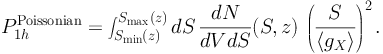 |
(36) |
On the other hand, the 2-halo term in Eq. (35) is obtained under the hypothesis that the fluctuations in the source distribution traces the fluctuations in the matter field, except for a bias factor bX(Y, z). That is the reason to include the linear power spectrum of matter fluctuations Plin in Eq. (35). Thus, even for point-like sources, the 2-halo term inherits a dependence on k.
The balance between the 1-halo and 2-halo terms determines the shape of PX(k, χ) and of Cℓ through Eq. (32). For a population of point-like sources that are very bright but scarce in number, P1hPoissonian usually dominates and it is difficult (if not impossible) to use the APS to extract information on their clustering. On the other hand, if the point-like emitters are very abundant, P1hPoissonian is smaller, allowing for some sensitivity to the 2-halo term. On the other hand, if the sources appear extended, the 1-halo is no longer Poissonian and it is suppressed above a certain scale associated with the typical size of the sources [51, 107, 406].
Following the formalism presented above, Refs. [52, 107] compute the APS of unresolved blazars. Blazars are characterized in Refs. [52, 107] by their gamma-ray luminosity (Y ≡ Lγ) which is assumed to correlate with the X-ray luminosity LX, see Sec. 2.2.1. The free parameters in the model are fitted to reproduce the abundance of sources detected by EGRET. Ref. [107] finds that the APS of unresolved blazars is within reach of the Fermi LAT and that it is dominated by the Poissonian 1-halo term for multipoles larger than a few. Similar results are obtained in Ref. [52].
Ref. [67] revises the predictions for the APS of unresolved blazars by modeling the differential source count distribution dN / dS as done in Ref. [18]. Eq. (36) is used to derive the intensity APS from dN / dS:
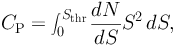 |
(37) |
where Sthr is the flux sensitivity threshold for point-like sources. dN / dS is assumed to be a broken power law, tuned to reproduce the measured abundance of blazars. Interestingly, the best-fit dN / dS corresponds to a model in which unresolved blazars exhibit an APS that is consistent with the value measured by the Fermi LAT in Ref. [66]. This suggests that blazars alone are able to explain the whole APS signal. The same best-fit model predicts that unresolved blazars can account only for ∼ 30% of the DGRB intensity reported by the Fermi LAT in Ref. [8] between 1 and 10 GeV.
The authors of Ref. [68] employ a more detailed model of the blazar population, based on the correlation between Lγ and LX and on a parametrization of their SED (see Ref. [19] and Sec. 2.2.1). They confirm the existence of a scenario in which blazars fit at the same time the Fermi LAT dN / dS and the measured APS. In this case, unresolved AGNs account for at most 4.3% of the DGRB intensity in Ref. [8] (in any energy bin). The constraints obtained in Refs. [67, 68] on the contribution of unresolved blazars to the DGRB intensity showcase how informative and complementary the study of gamma-ray anisotropies can be for the reconstruction of the composition of the DGRB.
The most recent estimate of the APS of blazars can be found in Ref. [63], where the authors consider three distinct AGN subclasses: i) FSRQs, ii) HSP BL Lacs and iii) a combination of LSP and ISP BL Lacs (see Sec. 2.2.1). Their Poissonian intensity APS is computed separately, according to Eq. (37). The dN / dS is taken from Ref. [22] for FSRQs and from Ref. [24] for the two classes of BL Lacs. They conclude that, as found previously, unresolved blazars can explain the whole APS signal, see Fig. 15. HSP BL Lacs are responsible for the largest fraction of the measured intensity APS: between 1 and 2 GeV, they account for 34.5−9.4+9.5% of the total APS signal and the fraction increases to 105−30+49% above 10 GeV.
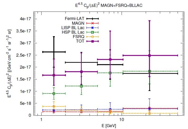 |
Figure 15. The angular power Cp(E) in units of E4.5 Cp(ΔE)−2 for MAGNs (red long-dashed points), a class of sources combining BL Lacs LSPs and BL Lacs ISPs (blue short-dashed), HSP BL Lacs (green dotted), FSRQs (yellow dot-dashed) and the total (violet solid) of all radio-loud AGNs. The APS measurement by the Fermi LAT Collaboration is also shown (black solid points). Taken from Ref. [63]. |
Ref. [63] also provides the first estimate of APS associated to MAGNs. It is computed from Eq. (37), assuming that the 2-halo term can be neglected. The properties of MAGNs are inferred from a modeling of the sources at radio frequencies, via the Lγ − Lr,core relation discussed in Sec. 2.2.2. Unresolved MAGNs are found to contribute to approximately 10% of the Fermi LAT APS (6.1% between 1 and 2 GeV and 16.7% above 10 GeV).
The APS of unresolved SFGs is computed in Ref. [145]. SFGs are described assuming that their luminosity is proportional to the product of their SFR and of gas mass. The model is tuned to reproduce the properties of the MW. A power law with an index of 2.7 is assumed in Ref. [145] as an universal energy spectrum (see Sec. 2.2.3). The APS is computed from Eqs. (34) and (35) assuming a bias factor of 1.11, independent of redshift and luminosity [412] (see also Ref. [399]). Contrary to the case of blazars or MAGNs, the APS of SFGs is not dominated by the Poissonian 1-halo term, at least below multipoles of few hundreds. As commented before, this is expected from a population of dim but very abundant sources. Thus, the signal may be used to constrain the clustering of SFGs. Unfortunately, the signal is overall too faint to contribute significantly to the APS detected by the Fermi LAT.
Refs. [37] and [38] performed Monte Carlo simulations of the APS signal expected from unresolved MSPs. Sources are modeled combining radio and gamma-ray data (see Sec. 2.2.4). The results of the two references differ from each other, due to the different models employed for the description of the MSPs: Ref. [38] assumes that the APS of MSPs is Poissonian and it finds that MSPs are responsible for no more than 1% of the APS measured by the Fermi LAT, while a larger fraction is allowed in the reference model considered by Ref. [37].
Among the other astrophysical components considered in Sec. 2.2.5, we mention that the clustering of Type Ia supernovae is considered in Ref. [413]: the authors find that unresolved supernovae can exhibit a moderately large APS but the emission peaks in the MeV energy range. Refs. [414, 209, 415, 202, 416, 107, 39] study the case of galaxy clusters. In particular, the model in Ref. [39] is tested against radio data and it proves that the intensity APS associated to galaxy clusters is expected to be two orders of magnitude lower than the APS measurement by the Fermi LAT.
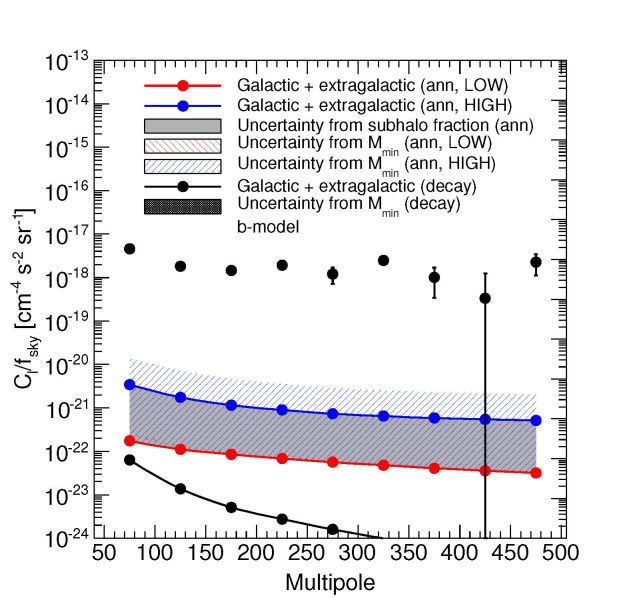 |
Figure 16. Total intensity APS of the gamma-ray emission from DM annihilation (color lines) or decay (black line) in extragalactic and galactic (sub)halos. The blue and red lines correspond to the LOW and HIGH subhalo boosts, respectively, so that the filled gray area between them corresponds to the uncertainty due to the subhalo boost, for a fixed value of Mmin. The red (blue) shaded area around the red (blue) solid line indicates the uncertainty in changing the value of Mmin from 1012 to 1 M⊙ / h, for the LOW (HIGH) case. The red-shaded area is very thin and difficult to see. The solid black line shows the prediction for a decaying DM candidate. The observational data points with error bars refer to the measurement of the APS between 2 and 5 GeV as given in Ref. [66]. The predictions refer to a DM particle with a mass of 200 GeV, an annihilation cross section of 3 × 10⁻²⁶ cm3 s−1 and annihilations entirely into b quarks (for annihilating DM) and to a mass of 2 TeV, a decay lifetime of 2 × 1027 s and decaying entirely into b quarks (for decaying DM). Taken from Ref. [62]. |
Turning to the case of gamma-ray emission induced by DM, the study of its angular anisotropies has also been traditionally considered as a very powerful strategy to single out the DM component of the DGRB [417]. Refs. [51, 52] adopt the Halo Model approach to determine the 1-halo and 2-halo terms from Eqs. (34) and (35), modeling the fluctuations in the gamma-ray emission produced by DM in extragalactic halos and subhalos. In Ref. [51] the authors neglect the contribution of subhalos, which is included in Ref. [52] assuming that the number of subhalos hosted by a halo with mass M scales with M. Their results suggest that, depending on the value of Mmin, the DM-induced fluctuation APS can be within reach of the Fermi LAT and that it can be larger than the APS expected for unresolved blazars. 37 Similar results are obtained also in Ref. [356], where only the 2-halo term is considered and modeled from N-body simulation data.
The analytic formalism of Refs. [51, 52] is extended to the case of Galactic DM in Ref. [54]. The DM halo of the MW is responsible only for large-scale anisotropies. On the other hand, the emission induced by Galactic subhalos can exhibit an APS that is even larger than the one from extragalactic DM structures. Results are tested in Ref. [54] against different parametrizations of the Galactic subhalo population. 38
Galactic and extragalactic DM signals are considered at the same time in Ref. [339]. For multipoles larger than few tens, the APS of the extragalactic component is dominated by the 1-halo term, which depends mainly on the amount of subhalos. In the fiducial model of Ref. [339], their luminosity is described by a power-law extrapolation of the cΔ(z, M) relation. As discussed in Sec. 2.3.1, this probably leads to an overestimation of the DM signal, which is, anyway, much smaller than the measured intensity APS. The latter can be used to derive upper limits on the annihilation cross section, excluding the region in the (mχ,⟨ σ v ⟩) plane associated with too large anisotropies. 39 The upper limits obtained in Ref. [339] exclude cross sections larger than 10−25 cm3 s−1 (5 × 10⁻²⁴ cm3 s−1) for a DM mass of 10 GeV (1 TeV), see the solid red line in Fig. 17. Similar results are obtained in Ref. [75].
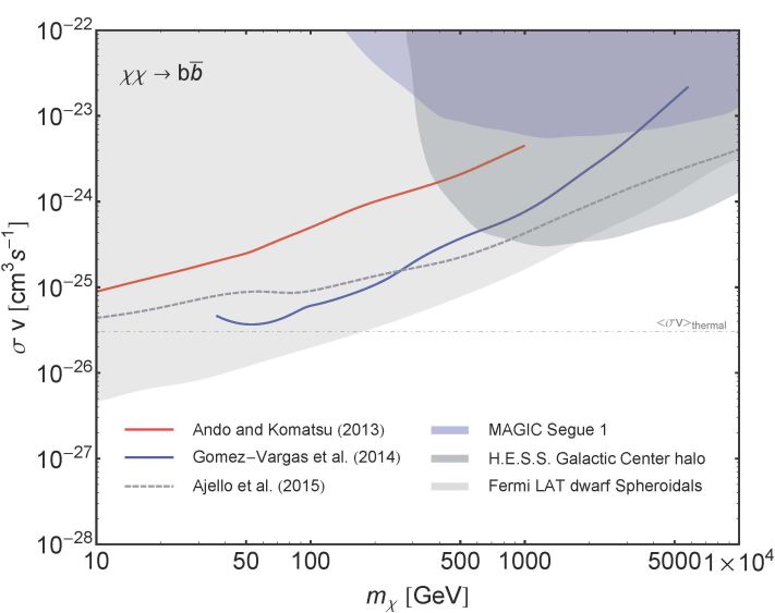 |
Figure 17. Upper limits obtained by considering the DGRB APS measured in Ref. [66]. The regions above the solid red and blue lines are excluded because the cumulative DM-induced emission would overproduce the APS of the DGRB. The solid red line is taken from Ref. [339] while the solid blue one is from Ref. [420]. The dashed gray line show the upper limits on ⟨ σ v ⟩ obtained by requiring that the DM-induced emission does not overproduce the DGRB emission measured in Ref. [9]. The limit is obtained in Ref. [25] by modeling the astrophysical DGRB contributors. The blue region indicates the region already excluded by the observation of the Segue 1 dwarf Spheroidal galaxy performed by the MAGIC telescope [368]. The dark gray region is excluded by the analysis performed by the H.E.S.S. telescope in Ref. [369] on the so-called “Galactic Center halo” region (assuming an Einasto DM density profile). The light gray region indicates the DM candidates not compatible with the combined analysis of Fermi LAT data from 15 dwarf Spheroidal galaxies [370]. The dash-dotted line marks the thermal annihilation cross section. |
Refs. [53, 55, 359] follows an alternative approach for the study of the anisotropies induced by Galactic DM subhalos. Instead of computing the APS analytically like in Refs. [51, 52, 54, 356, 339], Refs. [53, 359] simulate sky-maps of the gamma-ray emission expected from mock realizations of DM subhalos in the MW. The APS is, then, computed by means of the HEALPix package (see also Ref. [419]). In Ref. [366] the results of Ref. [53] on the APS of Galactic subhalos are combined with the predictions in Ref. [356] for the anisotropies of extragalactic DM to determine the sensitivity of Fermi LAT to the detection of a DM component in the DGRB through its APS.
Similarly, Ref. [55] employs a hybrid approach (inspired by Ref. [274]) in which Galactic DM subhalos are simulated only inside a sphere of radius rmax centered on the observer. The value of rmax is related to the distance beyond which subhalos become point-like. It is assumed that subhalos located further than rmax cumulatively generate a smooth emission. This is equivalent to assume that APS generated by subhalos beyond rmax is dominated by the 2-halo term.
Semi-analytic hybrid methods are used also in Refs. [56, 62] to compute the anisotropies in the emission of extragalactic DM structures. In this case, the distribution and properties of extragalactic (sub)halos with a mass larger than the mass resolution of the Millennium-II N-body simulation [343] are taken directly from the halo catalogs of the simulation. Mock sky-maps are generated by replicating the Millennium-II simulation box until it covers the region within z ∼ 2. 40 DM halos less massive than the resolution of Millennium-II are included assuming that they share the same clustering of those immediately above the mass resolution [56, 343]. Subhalos of extragalactic DM clumps are also accounted for considering multiple scenarios for their abundance and internal properties. Ref. [62] completes the prediction by modeling also the Galactic signal. The all-sky DM maps produced in Ref. [62] represent complete and accurate templates of the total DM-induced gamma-ray emission.
As in Sec. 2.3.1, the main sources of uncertainties in the DM-induced APS are the value of Mmin and the subhalo boost factor. Extreme scenarios are identified in Ref. [62] for both Mmin and the subhalo boost factor, bracketing their theoretical uncertainties. The effect of their variability on the intensity APS sums up to approximately two orders of magnitude, as it can be seen in Fig. 16. The red and blue lines show the intensity APS for two different prescriptions of the subhalo boost, labeled “LOW” and “HIGH”. The blue line is obtained following the prescription of Ref. [276], which employs power-law extrapolations for low-mass halos. On the contrary, the red line makes use of the model by Ref. [327], extended in Ref. [329]. The blue-shaded region shows the effect of changing Mmin on the HIGH scenario. 41 The black data points indicate the Fermi LAT APS measurement between 2 and 5 GeV. As in Ref. [339], the DM-induced emission is found to contribute only marginally to the measured APS.
In Ref. [420] the predictions of the HIGH case (blue line) are, then, used to derive upper limits on the DM annihilation cross section, shown as a solid blue line in Fig. 17. The upper limit reaches values as low as 3 × 10⁻²⁶ cm3 s−1 for mχ = 50 GeV, while going to 10−23 cm3 s−1 if the mass approaches the TeV scale. Fig. 17 also summarizes other constraints on ⟨ σ v ⟩ available in the literature. In particular, we plot the limit from the analysis of Ref. [25] of the DGRB intensity energy spectrum (dashed gray lines). The shaded regions indicate the areas already excluded by other indirect searches of DM, i.e. the observation of Segue 1 with MAGIC (blue), of the Galactic Center halo region with H.E.S.S. (dark gray) and the Fermi LAT combined analysis of dwarf Spheroidals (light gray). Fig. 17 proves that the study of the anisotropies of the DGRB can produce competitive upper limits on ⟨ σ v ⟩, but probably not as strong as those induced by the DGRB energy spectrum.
Ref. [62] also estimates the APS associated with a decaying DM candidate. In this case, as found also by Ref. [57], the predictions are subject to less theoretical uncertainties than for an annihilating DM candidate. In fact, the signal is less affected by the value of Mmin and there is no subhalo boost (see also Sec. 2.3.2). Yet, in decaying DM scenarios, DM halos yield a more extended emission. This is particularly true for Galactic subhalos which are still close enough not to be point-like. Thus, the APS is expected to decreases rapidly at high multipoles being, therefore, hard to detect. See, e.g., the black line in Fig. 16.
29 Moreover, as we will see in Sec. 3.1, the measurement of the DGRB anisotropies performed in Ref. [66] does not rely on the template fitting used in Ref. [9]. Back
30 Other observables have been used to quantify the anisotropies in the DGRB: Refs. [107, 398, 399] consider the 2-point correlation function in real space, while Ref. [400] relies on the nearest-neighbor statistics. Ref. [401] compares the number of “isolated” gamma-ray events with the “empty regions” in the sky. In this section, we focus only on the APS since it is the most commonly used technique. Back
31 http://healpix.jpl.nasa.gov/index.shtml Back
32 More recently, Ref. [405] presented an alternative method to estimate the error on Cℓ, developed specifically for scenarios like the DGRB, where the emission is affected by limited statistics. Back
33 In Eqs. (26) and (27) we are neglecting, for simplicity, possible cross-correlation terms between different components. Under the hypothesis that gamma-ray sources trace the same LSS of the Universe, these cross-correlation terms can contribute significantly to the total APS Cℓtotal and, thus, should be taken into account [52, 145, 339, 73, 406, 74]. Back
34 Since, as commented before, the APS is compatible with being constant in multipole, the whole APS can be completely characterized by just one number, that we refer to as Cp. Back
35 However, the large error bars and the fact that only 4 energy bins are available do not allow to exclude large-scale modulations or very localized peaks. Back
36 Compared to Eq. (1), we are neglecting the dependence on the spectral shape Γ. Back
37 The formalism was extended to include p-wave annihilations in Ref. [257]. Back
38 Ref. [54] and the majority of the references mentioned in this section do not consider the effect of baryons on the clustering of DM and, thus, on its anisotropy pattern. One exception is Ref. [418], which computes the APS expected by the so-called DM “mini-spikes”, i.e. DM overdensities induced by the presence of Intermediate-Mass Black Holes. The authors find that this scenario can lead to a significant increase in the amplitude of the DM-induced APS. Back
39 We note that, in general, the intensity APS associated with DM scales quadratically on ⟨ σ v ⟩. The study of anisotropies is, therefore, quite sensitive to a DM signal. Whether the upper limits on ⟨ σ v ⟩ derived from the Fermi LAT APS are more constraining than those from the DGRB intensity energy spectrum, will depend on the amplitude of the intrinsic fluctuations in the DM-induced gamma-ray emission. See also Fig. 17. Back
40 Beyond this distance, at the energies considered, the gamma-ray flux is almost entirely attenuated by the interaction with the EBL. Back
41 Changing Mmin has no effect on the red line (LOW case), see Ref. [62] for details. Back