


The subject of this section is the intensity energy spectrum of the DGRB. The first subsection (Sec. 2.1) summarizes the most recent measurement of this observable, i.e. the one performed by the Fermi LAT in Ref. [9]. The following subsections (Sec. 2.2 and Sec. 2.3) present the different source classes and emission mechanisms that have been proposed to interpret the observed emission. For each population we summarize how the DGRB energy spectrum has been used to learn about the properties of the gamma-ray emitters.
2.1. The new Fermi LAT measurement of the Diffuse Gamma-Ray Background
The Fermi LAT [78] on board the NASA Fermi satellite started its scientific operation on August 2008 and, since then, it has revolutionized our knowledge of the most violent phenomena in the Universe. The Fermi LAT covers 4 decades in energy, from few dozens of MeV up to the TeV regime. It has an unprecedented sensitivity (∼ 30 times better than its predecessor EGRET) and an extremely large field of view reaching almost one fifth of the sky. Its angular resolution is of about 0.8° at 1 GeV and better than 0.2° above 10 GeV. 3 Such superb capabilities allowed the discovery of hundreds of new gamma-ray sources and an impressive cartography of the Galactic CR-induced gamma-ray diffuse emission that reaches, for the first time, energies greater than 10 GeV [79].
In addition to these achievements, the analysis of 10 months of data delivered the first Fermi LAT measurement of the DGRB energy spectrum at Galactic latitudes, b, greater than 10 degrees [8]. Such a measurement was performed between 200 MeV and 102 GeV and it represents the third independent observation of the DGRB, after the one by the SAS-2 satellite in 1978 between 40 and 300 MeV [80] and that by EGRET between 40 MeV and 10 GeV in 1998 [6]. The energy spectrum of the DGRB as measured by the Fermi LAT in Ref. [8] is featureless and it can be well described by a single power law with a spectral index of 2.41 ± 0.05. This is significantly softer than both the DGRB initially reported by EGRET [6] and the revised estimate of Ref. [81] from the same data set. 4
More recently, a new measurement of the DGRB energy spectrum has been performed by the Fermi LAT [9]. The analysis used 50 months of data with |b| > 20°, it employed a dedicated event selection and it took advantage of improvements in the determination of the CR background and of the diffuse Galactic foreground. The measurement, denoted by red data points in Fig. 1, now extends down to 100 MeV and up to 820 GeV. It represents the most complete and accurate picture that we currently possess of the DGRB intensity. Interestingly, the DGRB now exhibits a high-energy exponential cut-off at 279 ± 52 GeV (for the baseline model of Galactic diffuse foreground used in Ref. [9]), and it is well described by a single power law with a spectral index of 2.31 ± 0.02 at lower energies. The cut-off is compatible with the attenuation expected from the interaction of high-energy photons with the EBL [82, 83, 84, 85, 86, 87, 88] over cosmological distances [25]. The largest systematic uncertainty (represented by the red shaded region in Fig. 1) ranges between a factor of ∼ 15% and 30% (depending on the energy range considered) and it comes from the modeling of the Galactic diffuse emission.
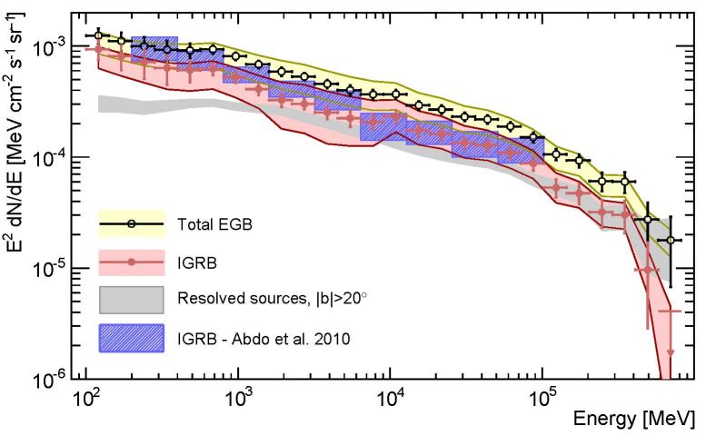 |
Figure 1. In red, the DGRB intensity energy spectrum, labeled “Isotropic Gamma-Ray Background (IGRB)” in the figure. Model A from Ref. [9] is used for the diffuse Galactic foreground. The spectrum is compared to the previous Fermi LAT measurement of the DGRB from Ref. [8] (blue bands) and to the total “Extragalactic Gamma-ray Background (EGB)” (black data points). The latter is defined here as the sum of the DGRB and of the resolved sources at |b| > 20° (shown in gray). The comparison shows that, above 100 GeV, ∼ 50% of the Extragalactic Gamma-ray Background is now resolved into individual LAT sources. Yellow and red shaded bands represent the systematic error associated with the uncertainties in the modeling of the Galactic diffuse emission. Taken from Ref. [9]. |
For the purposes of this review, it is convenient to briefly summarize here the main steps followed in Ref. [9] to measure the DGRB. Two different sets of selection cuts are applied to the gamma-ray data, optimized over different energy ranges, namely below and above 12.8 GeV. Different selection criteria are required because of the energy dependence in the composition of the CR-induced backgrounds and the way CRs interact with the detector. For the low-energy data sample, the all-sky Galactic diffuse emission is modeled as a sum of templates obtained with GALPROP 5 and the point-like sources are modeled following the information in the Second Fermi LAT catalog (2FGL). Additional templates are used to model subdominant contributions from the Loop I large-scale Galactic structure and from electrons interacting with the Solar radiation field through Inverse Compton (IC). A fully isotropic template is also included, in order to describe the DGRB and the residual CR contamination. The fit to the data determines the normalizations of the different templates and it is performed independently in each energy bin considered. At the highest energies, where the statistic is scarce, the normalizations of the templates for the Galactic diffuse emission are fixed to the best-fit values obtained at intermediate energies (between 6.4 and 51.2 GeV). The spectral shapes of their emission are also fixed to those predicted by GALPROP. Above 12.8 GeV, then, the normalizations of the point-like sources and of the isotropic template are the only free parameters in the fit.
Monte Carlo simulations are used to estimate the residual CR contamination. The energy spectrum of the DGRB is, finally, obtained by subtracting the CR contamination from the isotropic component determined in the template fitting. The systematic error induced by the imperfect knowledge of the Galactic diffuse emission is estimated by repeating the whole procedure for three benchmark models of Galactic foreground and for different values of the parameters controlling the propagation of CRs in the MW (see Ref. [9] for further details).
2.2. The astrophysical components of the Diffuse Gamma-Ray Background
In this section we describe the classes of astrophysical sources and emission mechanisms that have been proposed as contributors to the DGRB over the years. Well-established astrophysical populations, whose brightest members have been robustly detected, represent “guaranteed” components to the DGRB. They are discussed in Sec. 2.2.1, Sec. 2.2.2, Sec. 2.2.3 and Sec. 2.2.4, which are devoted, respectively, to blazars, MAGNs, SFGs and MSPs. Then, in Sec. 2.2.5, we turn to more speculative scenarios. We do not discuss the possibility of a DM-induced contribution to the DGRB, since that is the subject of the following section (Sec. 2.3).
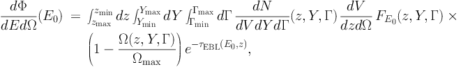
We start by presenting a formalism that will be adopted throughout the manuscript for the description of a generic population of sources. The sources are supposed to be characterized by a measurable quantity Y. In most cases Y will be the blue gamma-ray luminosity Lγ of the source but, in some instances, it will indicate another parameter such as, e.g., the mass of the galaxy or of the DM halo hosting the gamma-ray emitter. The differential gamma-ray flux dΦ / dEdΩ (i.e. the number of photons per unit area, time, energy and solid angle) expected from the unresolved objects in such a population can be written as follows:
 |
(1) |
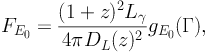
where z is the redshift and Γ is a parameter that characterizes the shape of the energy spectrum of the sources. The domain of integration will depend on the particular population considered. The factor dN / dVdYdΓ indicates the comoving number density of sources per unit Y and Γ, while dV / dzdΩ is the comoving volume per unit redshift and solid angle. The factor FE0(z, Y, Γ) is the gamma-ray flux (at energy E0) produced by the source identified by the value Y, located at redshift z and with an energy spectrum characterized by Γ. If sources are described by their gamma-ray luminosity (Y = Lγ), FE0 can be written as follows:
 |
(2) |
where DL(z) is the luminosity distance at redshift z and gE0(Γ) parametrizes the gamma-ray energy spectrum. For other choices of Y, the relation between Y and FE0 needs to be specified case per case.
Thus, the first line of Eq. (1) indicates the cumulative emission expected from all the sources located between zmin and zmax and with characteristics between (Ymin, Γmin) and (Ymax, Γmax). The quantity Ω(z, Y, Γ) is called sky coverage and it is defined as the area Ωmax surveyed by the telescope multiplied by the detection efficiency. It represents the probability for a source characterized by parameters (z, Y, Γ) to be detected and it encodes the sensitivity of the instrument, i.e. Ω(z, Y, Γ) is equal to zero if the source is too faint to be detected. It also accounts for any potential selection effect. An estimate of Ω(z, Y, Γ) for the high-latitude blazars in the first Fermi LAT catalog (1FGL) is provided in Ref. [8]. Then, the factor (1 − Ω(z, Y, Γ) / Ωmax) in Eq. (1) has the effect of selecting only the sources that remain undetected. Finally, the exponential e−τEBL(E0, z) accounts for the effect of the EBL attenuation.
It is also convenient to define a generic expression for the differential source count distribution dN / dS, i.e. the number of sources per unit solid angle and per unit flux S:
 |
(3) |
where S is the gamma-ray flux associated with the source characterized by (z, Y, Γ). 6 Note that the factor Ω(z, Y, Γ) / Ωmax has now the effect of selecting only the resolved objects. The number of sources (per solid angle) with a flux larger than S, i.e. the cumulative source count distribution N(> S), can be obtained by integrating Eq. (3) above S.
Blazars are among the brightest gamma-ray sources in the sky. They are interpreted as Active Galactic Nuclei (AGNs) with the relativistic jet directed towards the observer [89, 90]. The emission coming from the jet normally outshines the radiation associated with the accretion onto the supermassive Black Hole at the center of the nucleus. The Spectral Energy Distribution (SED) is bimodal: the low-energy peak is located between ultraviolet (UV) and radio frequencies and it corresponds to the synchrotron emission produced by the electrons that are accelerated in the jet. Instead, the high-energy peak reaches the gamma-ray band and it is produced by IC of the same population of synchrotron-emitting electrons. The seed photons for the IC emission come either from the synchrotron radiation itself (i.e., the so-called synchrotron self-Compton) or from the accretion disk (external Compton). Blazars can be divided in two categories: BL Lacs and Flat Spectrum Radio Quasars (FSRQs). Sources belonging to the first class have a nuclear non-thermal emission so strong that the rest-frame equivalent width of the strongest optical emission line is narrower than 5 Ȧ, while FSRQs have broader lines and a spectral index αr < 0.5 in the radio band. Blazars have also been classified according to the frequency of their synchrotron peak, νS [91, 92]: low-synchrotron-peaked (LSP) blazars have a peak in the infrared (IR) or far-IR band, (νS < 1014 Hz), intermediate-synchrotron-peaked (ISP) blazars for νS in the near-IR or UV (1014 Hz ≤ νS < 1015 Hz) and high-synchrotron-peaked (HSP) blazars for νS ≥ 1015 Hz, i.e. in the UV band or higher. From the study of the 886 blazars present in the Second Fermi LAT AGN catalog (2LAC) [93] it was confirmed that FSRQs (which are almost entirely LSPs) are generally brighter than BL Lacs. Also, it was possible to determine a correlation between the steepness of their energy spectrum (in the gamma-ray band) and the position of the synchrotron peak, suggesting that FSRQs (with a low νS) have softer spectra than BL Lacs [93].
Since the EGRET era, blazars were suspected to play a significant role in explaining the DGRB emission, with estimates ranging from 20% to 100% [94, 10, 11, 12, 13, 15, 95, 30, 16]. Fewer AGNs were known before the Fermi LAT (66 in the third EGRET catalog [96], mainly FSRQs), preventing reliable population studies to be performed entirely at gamma-ray energies. Predictions for the emission of unresolved blazars were obtained by means of well-established correlations between the gamma-ray luminosity Lγ and the luminosity at lower frequencies, either in the radio or in the X-ray band [94, 11]. Thus, the strategy followed in these early works was to characterize the blazar population in those low-frequency regimes, where the statistical sample was much larger, and then export the information up to the gamma-ray range by means of the aforementioned correlation between luminosities.
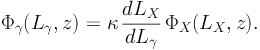
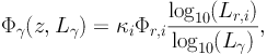
Ref. [16] considers the correlation between Lγ and the luminosity in X-rays, LX. The Lγ − LX connection is a consequence of the relation between the emission of the jet (which can be linked to Lγ) and the mass accretion onto the supermassive Black Hole [97, 98, 99, 100]. This, in turn, correlates with the X-ray luminosity of the accretion disk LX. Ref. [16] considers Lγ as the Y-parameter in Eqs. (1) and (3). The dependence on Γ in the factor dN / dV dLγ dΓ is taken care of by the so-called “blazar sequence” [101, 102, 103], which predicts how the shape of the blazar SED changes as a function of their luminosity. Then, integrating Eq. 1 over Γ, the blazar sequence selects, for each Lγ, the only SED compatible with Lγ. On the other hand, dN / dV dLγ is the gamma-ray luminosity function (LF), Φγ(z, Lγ). Given the Lγ − LX relation, Φγ(z, Lγ) can be inferred from the X-ray LF ΦX(LX, z):
 |
(4) |
The factor κ indicates the fraction of AGNs observed as blazars and a parametrization for ΦX(z, LX) is available in Refs. [104, 105, 106]. X-ray AGNs are found to evolve positively (i.e. they are more abundant as redshift increases) until a certain redshift peak zc, above which the X-ray LF decreases [104, 105, 106]. It was found that allowing zc to vary with LX (i.e., what is called a luminosity-dependent density evolution) provides a better description of the blazars observed by EGRET than other evolution schemes, e.g., pure luminosity evolution or pure density evolution [13].
Parameter κ in Eq. (4) is left free in the analysis of Ref. [16], together with the faint-end slope γ1 of the X-ray LF and the proportionality coefficient between Lγ and LX. 7 These parameters are determined by a maximum-likelihood fit to the differential source count dN / dS of the blazars detected by EGRET. The best-fit model is, then, used to determine the contribution of unresolved blazars to the DGRB through Eq. (1). Ref. [16] finds that unresolved blazars can explain approximately 45% of the DGRB measured by EGRET in Ref. [7] at 100 MeV.
Similar results are obtained in other works that follow the same formalism: Refs. [13, 107, 52] also consider a luminosity-dependent density evolution for the X-ray LF but they assume a common power-law energy spectrum at gamma-ray frequencies, instead of the SED predicted by the blazar sequence. In Ref. [19] the formalism outlined before is fitted to both the blazar dN / dS computed from the 1FGL [108] and to the first Fermi LAT measurement of the DGRB in Ref. [8] (see also Ref. [109]). The result of the fit proves that it is possible to explain both observables with one single population of blazars. 8 Their predictions are re-calibrated in Ref. [68], where the model is fitted against the 1FGL dN / dS and the Fermi LAT measurement of the DGRB auto-correlation APS of anisotropies from Ref. [66] (see Sec. 3). Ref. [68] finds that the DGRB intensity energy spectrum and the auto-correlation APS cannot be simultaneously explained in terms of unresolved blazars, since a model that fits both the abundance of resolved blazars (i.e., their dN / dS) and the DGRB intensity energy spectrum would exceed the measured auto-correlation APS. Alternatively, unresolved blazars can reproduce the measured anisotropies but, then, their emission only accounts for a maximum of 4.3% of the DGRB intensity in Ref. [8], above 1 GeV.
Instead of using the Lγ − LX correlation discussed above, Ref. [11] relates Lγ to the radio luminosity, Lr. The gamma-ray LF is inferred from the radio LF, similarly to what done in Eq. (4). The radio LF is taken from Ref. [110]. A power-law energy spectrum is assumed at gamma-ray frequencies, while the distribution of spectral indexes dN / dΓ is calibrated to reproduce the sources detected by EGRET. Ref. [11] finds that unresolved blazars can fit reasonably well the EGRET DGRB energy spectrum reported in Ref. [6]. Other works exploit the Lγ − Lr relation with similar findings: Ref. [111] determines the properties of the blazar population by fitting their measured radio LF (assuming it follows a pure luminosity evolution), while in Ref. [20] the fit is performed with the cumulative source distribution N(> S) of 1FGL blazars. The authors of Ref. [20] also caution about the use of the sky coverage determined in Ref. [18], since it may be affected by systematic uncertainties in the low-flux regime due to low statistics.
With the advent of the Fermi era, direct population studies at gamma-ray frequencies became possible, without the need to rely on correlations with lower frequencies. Following the formalism of Eqs. (1) and (3), in Ref. [18] the Y parameter is taken to be the flux S above 100 MeV. The energy spectra of the blazars are assumed to be power laws with indexes Γ characterized by a Gaussian probability distribution independent of S. The gamma-ray LF dN / dV dS is combined with the factor dV / dz dΩ in Eq. (3) into dN / dz dS dΩ, which is assumed to be the same for all the sources considered and to depend on S as a broken power law. No correlation with other frequencies is required. The parameters of the broken power law (as well as the mean and standard deviation of the Gaussian distribution for Γ) are inferred through a maximum-likelihood fit to the blazars in the 1FGL with |b| > 20°. The best-fit point has a break at S = (5.99 ± 0.91) × 10−8 cm−2 s−1 and slopes of 1.58 ± 0.08 and 2.44 ± 0.11 above and below the break [18]. The model is, then, used to determine the cumulative emission of unresolved sources. Results indicate that unresolved blazars (with Smin = 0) account for 23% of the DGRB detected by Fermi LAT in Ref. [8].
Ref. [22] improves the analysis in Ref. [18], attacking one of its main limitations, i.e. the fact that the broken power law considered for dN / dz dS dΩ is assumed a priori and it is not inferred from a specific evolution scheme. In Ref. [22], the analysis is restricted to FSRQs: sources are identified by their Lγ (i.e., Y ≡ Lγ), their redshift and the slope of the power-law fit to their energy spectrum. dN / dV dLγdΓ is split into the gamma-ray LF and the spectral index distribution dN / dΓ. The former is described by a parametric expression inspired by the results in the radio and X-ray bands, while a Gaussian distribution is assumed for dN / dΓ, with no dependence on Lγ. A maximum-likelihood fit is performed to determine the parameters of the model. 186 FSRQs in the 1FGL and with |b| ≥ 15° are considered in the fit. Results establish that FSRQs evolve positively until a zc that depends on Lγ, i.e. a luminosity-dependent density evolution performs better than other evolution formalisms. The best-fit model corresponds to an unresolved emission which accounts for 9.3−1.0+1.6 % of the Fermi LAT DGRB in Ref. [8], between 0.1 and 100 GeV (see Fig. 2). 9 The contribution peaks below the GeV scale and it becomes more subdominant at higher energies.
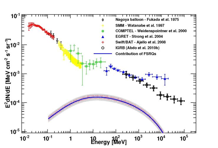 |
Figure 2. Contribution of unresolved FSRQs to the DGRB as determined by integrating the LF coupled to the SED model derived in Ref. [22]. The red hatched band around the best-fit point prediction (solid blue line) shows the 1σ statistical uncertainty, while the gray band represents the systematic uncertainty. Note that, in the figure, the DGRB measured by the Fermi LAT in Ref. [8] (black data points) is refereed to as “IGRB”. Taken from Ref. [22]. |
Performing a similar population study for BL Lacs is hampered by the fact that it is more difficult to obtain a measure of spectroscopic redshift for these objects due to the lack of strong emission lines: indeed, approximately 55% of the BL Lacs in the 2LAC do not have an associated z. This issue is somehow alleviated in Ref. [23] by considering photometric redshift estimates [113], lower [114] or upper limits on z [113, 114] and host-galaxy spectral fitting [114]. The 211 BL Lacs studied in Ref. [23] are taken from Ref. [18] and analyzed by means of the same pipeline applied in Ref. [22] to FSRQs: the Y parameter in Eq. (1) is again Lγ but the mean of the Gaussian distribution of spectral indexes depends now linearly on log10(Lγ). Only sources with Lγ ≥ 7 × 1043 erg s−1 are considered. The best-fit model suggests that the number density of faint BL Lacs (probably HSPs) decreases with redshift, while BL Lacs with Lγ ≥ 1045.8 erg s−1 are more numerous at large redshift, i.e. more similar to the positive evolution FSRQs. The redshift estimates adopted for the BL Lacs without spectroscopic information are crucial to constrain the evolution of their LF. Results indicate that unresolved BL Lacs contribute to 7.7−1.3+2.0 % of the Fermi LAT DGRB in Ref. [8], between 0.1 and 100 GeV. Due to the large density of low-luminosity hard sources at low redshift, the emission of unresolved BL Lacs is expected to be harder than that of FSRQs and, thus, BL Lacs may play a more significant role at higher energies.
This hypothesis was tested by Ref. [24], where the authors considered a set of 148 BL Lacs with redshift and synchrotron peak frequency νS obtained from the 2FGL [115]. Their model for the gamma-ray LF is fitted to the observed cumulative source distribution N(> S), the gamma-ray LF and the redshift distribution dN / dz of the detected sources. The energy spectra of the sources are obtained from a combination of Fermi LAT and Imaging Air Cherenkov Telescopes data. A luminosity-dependent density evolution is found to provide the best fit to the data. Pure power laws, log-parabolae and power laws with exponential cut-offs are considered as possible SEDs, with the last one corresponding to the most accurate description of the BL Lacs in the sample. The sources were considered as either one single population, or split into HSPs and a second sub-class including ISPs and LSPs. In their best-fit model, HSPs dominates the dN / dS below S = 5 × 10⁻⁹ cm−2 s−1 and their SED extends to much higher energies than in the ISP+LSP class (the best-fit cut-off energy is 910 GeV for HSPs and 37 GeV for the class of ISPs and LSPs). That is the reason why the cumulative emission from HSPs (computed from Eq. (1) above Lγ ≥ 1038 erg s−1) can extend up to very high energies and it is able to explain the whole DGRB emission reported in Ref. [112] above few tens of GeV (see Fig. 3). Between 0.1 and 100 GeV, unresolved BL Lacs account for ∼ 11% of the Fermi LAT DGRB in Ref. [112], in agreement with Ref. [23].
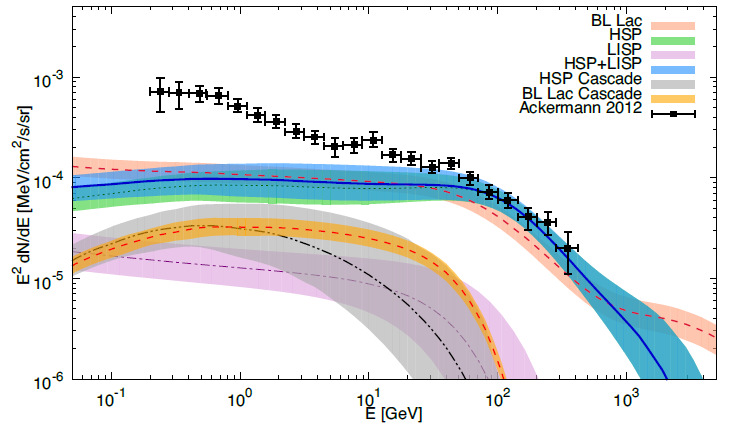 |
Figure 3. Diffuse gamma-ray emission from unresolved BL Lacs. Predictions for the best-fit model in Ref. [24] are shown embedded in their 1σ uncertainty bands: the summed contribution from LSPs and ISPs is plotted by means of the purple dot-dashed line and the purple band, the one from HSP BL Lacs by the green band and green dotted line (almost overlapped with the blue band), the one from the sum of the two by blue band and solid blue line and the contribution from BL Lacs considered as a unique population is depicted by the pink band and dashed pink line. The DGRB data are taken from Ref. [112] and are displayed as black points. The gray band and double-dot-dashed black line (orange band and dashed red line) represent the cascade emission from the HSP BL Lacs (the whole BL Lac population). Taken from Ref. [24]. |
Ref. [25] repeated the analysis of Ref. [23] on a sample of 403 blazars from 1FGL, this time considering both FSRQs and BL Lacs as one single population by allowing the spectral index distribution to depend on Lγ. A double power-law energy spectrum, proportional to [(E0 / Eb)1.7 + (E0 / Eb)2.6]−1, is assumed and the energy scale Eb is found to correlate with the index Γ obtained when the SED is fitted by a single power law. The same LF used in Ref. [23] and based on a luminosity-dependent density evolution is implemented in Ref. [25], together with other evolution schemes. They all provide an acceptable description of the blazar population, even if the luminosity-dependent density evolution is the one corresponding to the largest log-likelihood. The predicted cumulative emission of blazars (FSRQs and BL Lacs, resolved and unresolved) can be seen in the Fig. 4 as a dotted blue band, compared to the total emission from resolved and unresolved sources taken from Ref. [9] (labeled “EGB” here, red data points). Blazars (both resolved and unresolved) accounts for the 50−11+12 % of the total emission from resolved and unresolved sources, above 100 MeV. Unresolved blazars, on the other hand, are responsible for approximately 20% of the new Fermi LAT measurement of the DGRB in Ref. [9], in the 0.1-100 GeV energy band.
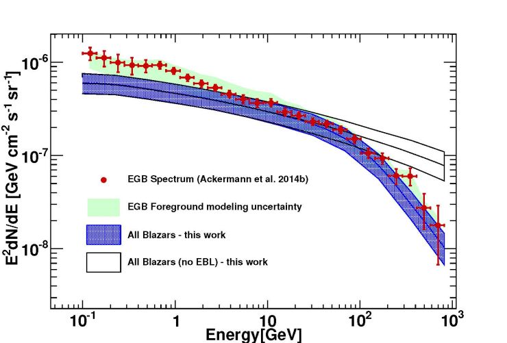 |
Figure 4. Diffuse emission arising from blazars (with or without EBL absorption), in comparison with the intensity of the total emission from sources (both resolved and unresolved), called here “EGB” (red data points, from Ref. [9]). Taken from Ref. [25] |
2.2.2. Misaligned Active Galactic Nuclei
Under the AGN unification scenario, the parameter that discriminates among different classes of AGNs is the viewing angle [89]. A value of 14° separate blazars (with the jet pointing towards the observer) from non-blazars, i.e. MAGNs. Among MAGNs it is possible to further distinguish between radio galaxies (with a viewing angle larger than 44°) and radio quasars [116]. Radio galaxies are classified either as Fanaroff-Riley Type I or Type II (FRI and FRII, respectively) according to their morphology [117]. The emission of FRIs peaks at the center of the AGN and it is dominated by two-sided decelerating jets. On the other hand, FRIIs are brighter and they are characterized by edge-brightened radio lobes with bright hotspots, while jets and core (when detected) are subdominant. FRIs and FRIIs are normally interpreted as the misaligned counterparts of BL Lacs and FSRQs, respectively. Indeed, the detection of MAGNs in the 1FGL and 2FGL confirms that, similar to the case of BL Lacs and FSRQs, FRIs have harder spectra than FRIIs [118].
The mechanisms of gamma-ray production in MAGNs are less clear than for blazars: the SED exhibits a bimodal structure, with the low-frequency peak due to synchrotron radiation, while at higher energies, the bulk of gamma-ray emission may be due to synchrotron self-Compton [119]. External IC may also contribute [120]. If present, external IC would be localized within one parsec from the center of the AGN, while synchrotron self-Compton emission is produced outside that region [119, 120]. Furthermore, spatially coincident with the radio lobes, there may also be emission from IC off the Cosmic Microwave Background (CMB) [27, 26] (see the discussion at the end of this section).
With no Doppler boost, MAGNs are expected to be less bright but more abundant than blazars, making them potentially important contributors to the DGRB [28]. 15 MAGNs were reported in Ref. [118], precluding the possibility of deriving their gamma-ray LF directly from gamma-ray observations, as done with blazars. Yet, the LF of MAGNs is well known at radio frequencies. As done in the previous section, once a correlation between their radio and gamma-ray luminosities is established, it is possible to deduce the gamma-ray properties of MAGNs by studying the sources in the radio band.
Ref. [28] considers Lγ (between 0.1 and 10 GeV) for 10 MAGNs detected by the Fermi LAT in Ref. [118]. The author studies the possibility of a linear correlation between log10(Lγ) and log10(Lr), where Lr is the radio luminosity. The slope of the observed correlation is very similar to the one found by Ref. [121] for blazars. Then, Φγ(z, Lγ) is determined in terms of the radio LF, Φr(z, Lr), as Φγ(z, Lγ) = κ Φr(z, Lr) dLr / dLγ. This is similar to Eq. (4) for blazars. Ref. [28] takes Φr from Ref. [122] and the value of κ is tuned to reproduce the number of sources observed by the Fermi LAT. All MAGNs are assumed to share the same energy spectrum, i.e. a power law with an index of 2.39. Such a value is the mean spectral index among the 10 MAGNs considered. The emission from unresolved MAGNs is, finally, estimated from Eq. (1), for Lγ ≥ 1039 erg s−1. The result indicates that ∼ 25% of the DGRB measured by Fermi LAT in Ref. [8] above 100 MeV can be explained in terms of unresolved MAGNs.
Ref. [29] improves the analysis in Ref. [28] by properly estimating the uncertainties involved: the authors consider Lγ (defined above 100 MeV) of 12 MAGNs in the 2FGL and the correlation with Lr at 5 GHz. They make use of the total radio luminosity, Lr,tot, and the so-called “radio core luminosity” Lr,core, defined as the emission from the central arcsecond-scale region of the source. Both the log10(Lγ) − log10(Lr,core) and log10(Lγ) − log10(Lr,tot) relations are considered. The gamma-ray LF is inferred from the radio LF as follows:
 |
(5) |
where i stands for “total” or “core”. 10 If Lr,tot is used, Φr,tot is taken from Ref. [122]. On the other hand, it is not possible to build the core radio LF directly from radio observation, due to the scarce data available [123]. In Ref. [29], a relation is assumed between Lr,core and Lr,tot [124], so that Φr,core can be derived from Φr,tot. The factor κi in Eq. (5) is tuned to reproduce the number of observed MAGNs. Different values for κ are obtained in Ref. [29], depending on which LF is considered (total radio or core radio) and on how the uncertainties in the log10(Lγ) − log10(Lr, i) correlations are treated. Finally, the emission from unresolved MAGNs is computed as in Eq. (1), assuming a Gaussian distribution for the spectral indexes. The results (for Lγ > 1041 erg s−1) are summarized in Fig. 5. For the best-fit model, the contribution of MAGNs accounts for ∼ 25% of the Fermi LAT DGRB in Ref. [8] above 100 MeV. The value agrees very well with that given in Ref. [28]. Yet, in Ref. [29], the prediction is embedded in an uncertainty band with a size of almost one order of magnitude. Such large uncertainty mainly comes from the possible different values for κ.
 |
Figure 5. Diffuse gamma-ray flux due to MAGNs as a function of the gamma-ray energy. The dashed black line is obtained from the best-fit to the Lr,core − Lγ correlation. The cyan shaded area is derived by allowing for the uncertainty on the Lr,core − Lγ correlation and by including all the models that are less than 1σ away from the best-fit point. The green band corresponds to the case with κ = 1 at 1σ confidence level. The red dot-dashed curve shows the diffuse flux obtained when assuming a correlation between the total radio luminosity and the gamma-ray luminosity. The black squares corresponds to the DGRB measured by the Fermi LAT in Ref. [8] and the magenta dashed curve represents the best-fit to the data. Taken from Ref. [29]. |
Given the complex morphology of the emission in radio galaxies, it is possible that different regions in the source emit gamma rays which are not accounted for by the analyses presented above. Ref. [27] considers a scenario in which the non-thermal electrons responsible for the synchrotron emission in the radio lobes of FRIIs could emit gamma rays by IC off the CMB. Indeed, gamma-ray emission spatially coincident with the radio lobes of Centaurus A has been recently observed by the Fermi LAT [125]. Such a component would peak at around 1 MeV and could explain up to 10% of the DGRB in Ref. [8] below 1 GeV.
Similarly, Ref. [26] considers the X-ray-emitting kpc-scale jets of FRIs as possible contributors to the DGRB. The established synchrotron origin of those X-rays suggests that the same non-thermal electrons could also emit gamma rays through IC with the ambient photons of the host galaxy. However, even assuming this is common for all FRIs, the contribution adds up to only ∼ 1% of the DGRB reported in Ref. [7].
The majority of the gamma-ray emission detected by the Fermi LAT is associated with the MW [79]. This diffuse Galactic foreground is produced by the interaction of Galactic CRs (mainly protons and electrons) with the Galactic interstellar medium and interstellar radiation field. Other SFGs similar to the MW are expected to shine in gamma rays thanks to the same emission mechanisms. Up to now, the Fermi LAT has only detected a few SFGs other than the MW: M31 and M33 [126], the Large and Small Magellanic Clouds [127, 128] in the Local Group and the Circinus Galaxy [129], M82, NGC 253 [130, 131], NGC 1068 and NGC 4945 [33]. Ref. [132] also reported the detection of gamma-ray emission from NGC 2146. Being intrinsically faint but numerous, SFGs are expected to contribute significantly to the DGRB.
Massive stars in SFGs emit the majority of their light in the UV band. The emission is then absorbed by interstellar dust and re-emitted as IR light. The IR luminosity can be used as a good tracer of the star-forming rate (SFR) ψ, i.e. the amount of mass converted in stars per unit time [33]. The same massive stars finally explode into core-collapse supernovae, leaving behind supernova remnants which are considered to be the main sources of accelerated CRs on galactic scales [134]. The leptonic component of these CRs is responsible for the synchrotron radio emission observed from SFGs and they may also contribute at gamma-ray frequencies when interacting with the interstellar radiation field of the host galaxy (through IC or bremsstrahlung). However, such leptonic gamma-ray emission is expected to be subdominant with respect to the hadronic one [35], since CR protons have an intrinsically larger injection rate than CR electrons [135, 34]. Hadronic gamma-ray emission mainly comes from inelastic interactions of CR protons with the nuclei of the interstellar medium, producing neutral pions that decay into gamma rays with an energy spectrum that peaks at around 300-400 MeV.
The so-called “initial mass function” determines the relative number of stars produced in any star-formation event in a galaxy, as a function of the stellar mass [136, 137]. Under the assumption of an universal high-mass end of the initial mass function, the SFR of a galaxy is proportional to the rate of supernova explosions and, thus, to the CR abundance and the CR-induced emission [138, 34]. Then, it is expected that, in a generic galaxy, the gamma-ray and radio luminosities (both associated with CRs) are correlated with the IR emission, which depends on the SFR.
The cumulative gamma-ray flux produced by IC of CR electrons in
all SFGs at all redshifts is computed in Ref.
[35].
In this work, the emission of a generic galaxy is modeled based on a
template which is tuned to reproduce the emission of the MW. The
cumulative gamma-ray flux depends on the abundance of SFGs. Ref.
[35]
assumes that, at a certain redshift, the total emission scales as the
so-called cosmic SFR
 ⋆(z), i.e. the mass
converted to stars per unit time and comoving volume:
⋆(z), i.e. the mass
converted to stars per unit time and comoving volume:
 |
(6) |
where dN / dVdψ is the comoving density of galaxies
per unit SFR. Parametric fits for
⋆(z) are available from the
observation of the total luminosity density at various wavelengths
[139,
140,
141].
Ref.
[35]
finds that the IC-induced emission is always subdominant with respect to
the hadronic one. The two become comparable only above 100 GeV.
Indeed, the majority of the studies on the SFGs focus on their hadronic emission and they neglect the contribution from primary electrons. The hadronic gamma-ray luminosity of a SFG, as a function of the observed energy E0, can be written as follows:
 |
(7) |
where Eem is the energy in the emitter frame, Γπ0 → γγ is the pionic gamma-ray production rate per interstellar hydrogen atom and nH is density of hydrogen atoms in the interstellar medium [31, 20]. Integrated over the volume of the medium, NH gives the total number of hydrogen atoms, which can be expressed in terms of the total interstellar gas mass Mgas in the galaxy as XH Mgas / mp. XH ∼ 0.7 is the hydrogen mass fraction and mp is the mass of the proton. As for Γπ0 → γγ in Eq. (7), it is the product of the flux Φp of CR protons (averaged over the volume of the galaxy) and the cross section for the production of gamma rays [142, 143].
The distribution and propagation of CR protons is governed by the diffuse-loss equation, which depends on their injection rate, diffusion, energy losses and possible inelastic interactions (see Ref. [34] for a recent review). Different scenarios are possible depending on the strength of those terms. Here we only mention two possibilities that provide good descriptions to different typologies of galaxies. The first is the so-called escape regime and it corresponds to a situation in which the energy losses of CR protons are dominated by their escape from the diffuse region of the galaxy. An equilibrium is reached between the energy losses and the acceleration of CR protons so that their flux is proportional to the product of the SFR of the galaxy and the CR escape path-length, Λesc: Φp ∝ Λesc ψ. Consequently, Lγ ∝ Mgas ψ [144, 145, 31]. The escape regime provides a good description of the diffuse foreground of the MW. This motivates the use of the gamma-ray production rate of the MW, Γπ0 → γγMW, to normalize the proportionality relation between Lγ and Mgas ψ. Then Eq. (7) becomes:
 |
(8) |
where ψMW is the SFR of the MW. This relation provides a good description of the so-called quiescent or normal SFGs, characterized by properties similar to those of the MW.
The second scenario considered for the modeling of SFGs is the so-called calorimetric regime: in this case the energy losses of CR protons is mainly due to their inelastic interactions. This means that protons lose all their energy into pions and SFGs act effectively as calorimeters. Their gamma-ray lumonisity, then, can be computed from the amount of energy available to CRs. Under the paradigm that supernova remnants are the primary source of CRs, the energy available in the form of CRs for a calorimetric SFG is proportional to the supernova rate, multiplied by the energy ESN released per supernova and by the fraction η of that energy going into CR protons (i.e. the so-called acceleration efficiency) [138, 33]. In turn, the supernova rate is proportional to the SFR, so that, finally,
 |
(9) |
Starburst galaxies are well modeled as proton calorimeters: normally brighter and less numerous than quiescent galaxies, starburst ones are characterized by at least one region undergoing intense star formation. This is often induced by major merger events or by bar instabilities, leading to a large gas density [146].
Several works analyze quiescent and starburst SFGs separately. Refs.
[144,
145,
31],
e.g., focus on quiescent galaxies. Their contribution to the DGRB is
computed by using a formalism similar to Eq. (1), where
Lγ is considered as the
Y-parameter. Then, by means of Eq. (8),
Lγ is written as a function of
Mgas and ψ. In Refs.
[144,
145],
the former is factorized out of the integral in
dLγ in
Eq. (1), assuming that Mgas only depends on
redshift. The integration in dLγ now only
depends on the SFR and it amounts to the cosmic SFR
⋆(z) in Eq. (6).
The net result is that the cumulative emission of quiescent SFGs scales
with redshift as the product of
⋆(z) and the average amount of
gas. Refs.
[144,
145]
take ⋆(z) from Refs.
[139,
140],
respectively, and derive the average
gas mass assuming that the total baryonic mass of a galaxy (stars and gas)
remains constant time and that it can be computed de-evolving backwards the
cosmic history of the SFR density
[144,
145].
They find that quiescent SFGs can contribute significantly to the DGRB,
especially below 1 GeV, but they are only subdominant at higher energies.
Ref. [31] assumes the same formalism than Ref. [144] but it relates the gas content of a galaxy to its SFR, using the following relation:
 |
(10) |
This is obtained by the so-called Kennicutt-Schmidt law [147, 148], which links the surface density of star formation to that of the gas. Then, the integration over Lγ in Eq. (1) is converted into one in SFR. In turn, the SFR is related to the IR luminosity, LIR, assuming a direct proportionality between the two [149]. The contribution of SFGs now depends on the IR LF, ΦIR. Ref. [31] considers the IR LF from Ref. [150]. Results are provided for both a pure luminosity evolution and a pure density evolution for ΦIR. The difference between the two prescriptions amounts to approximately a factor of 2 (see the dashed and long-dashed lines in Fig. 6). An intermediate scenario that mediates between the two evolution schemes indicates that unresolved SFGs account for ∼ 50% of the DGRB intensity reported in Ref. [8] below 10 GeV. Above that energy, the contribution of SFGs goes down rapidly due to the softness of the energy spectrum assumed, i.e. a power law with a slope of 2.75.
Ref. [20] proposes two alternatives to estimate Mgas: in the first one, the gas mass is not obtained from Eq. (10) but taken to be some fraction of the stellar mass M⋆. The latter can be constrained by combining the findings of Refs. [151, 152]. In the second scenario, the mean gas mass is assumed to scale with the cosmic SFR divided by a parameter linking the SFR to the density of clouds of molecular hydrogen [153, 20]. The two methods differ by approximately a factor of 10 in their predictions for the contribution of SFGs to the DGRB. In the second one, SFGs are able to account for the whole DGRB of Ref. [8] between 200 MeV and 1 GeV.
Starburst SFGs have also been considered: Ref. [138] works under the hypothesis that these objects are in the calorimetric regime. From Eq. (9), their gamma-ray luminosity is proportional to the SFR which, in Ref. [138], is related to the IR luminosity. Thus, the total gamma-ray emission from unresolved starburst SFGs can be obtained simply by rescaling the total diffuse extragalactic IR background taken, e.g., from Ref. [154]. Unresolved starburst galaxies are found to account for ∼ 10% of the DGRB detected by EGRET in Ref. [7], at least at the GeV scale (see the double-dotted-dashed line in Fig. 6). The main uncertainty affecting this prediction stems from the unknown starburst fraction, i.e. the fraction of the IR background emission associated with starburst galaxies in the calorimetric regime. Observations suggests that such a fraction is quite low at z = 0 but that it can approximate to 1 at earlier epochs, when the star formation is much more efficient [155, 156]. However, see also Refs. [157, 20, 158, 34] for different values.
 |
Figure 6. Estimated contribution of unresolved SFGs (both quiescent and starburst) to the DGRB emission measured by the Fermi LAT (black points, taken from Ref. [8]). Two different spectral models are used: a power law with a photon index of 2.2 (red line), and a spectral shape based on a numerical model of the global gamma-ray emission of the MW [135] (white line, inside gray band). The shaded regions indicate combined statistical and systematic uncertainties. Several other estimates for the intensity of unresolved SFGs are shown for comparison. For the double-dotted-dashed line starburst galaxies are treated as calorimeters of CR nuclei as in Ref. [138]. Ref. [31] (dashed and long-dashed line) considers the extreme cases of either pure luminosity and pure density evolutions. The solid black line shows predictions from Ref. [32], obtained from simulated galaxies and semi-analytical models of galaxy formation. Two recent predictions from Ref. [20] are plotted by dotted and dash-dotted black lines: the former assumes a scaling relation between IR and gamma-ray luminosities and the latter uses a redshift-evolving relation between the gas mass and the stellar mass of a galaxy. Taken from Ref. [33]. |
Both quiescent and starburst SFGs are modeled at the same time in Ref. [32]. The relations between Lγ and ψ Mgas and between Lγ and ψ for quiescent and starburst SFGs respectively (see Eqs. (8) and (9)) are determined by fitting the results of 4 SFGs detected by the Fermi LAT. On the other hand, the abundance of galaxies is inferred from simulated galaxy catalogs [159, 160]. Starburst SFGs are found to be always subdominant and the total (quiescent and starburst) gamma-ray emission is between 5.4% and 9.6% of the DGRB intensity reported by the Fermi LAT in Ref. [8] above 100 MeV (see the black solid line in Fig. 6).
In Ref.
[34]
the authors model the emission from the MW and
from M82, which are considered as templates of quiescent
and starburst SFGs, respectively. The results are used to determine
Lγ for the two typologies of SFGs. Their total
emission is assumed to evolve with redshift following
⋆(z), modulated by functions
fi(z) (where i
stands for either “starburst” or
“quiescent”) that fix the relative abundance of the two
sub-classes. They find that SFGs can be responsible from 4% to 76% of
the DGRB of Ref.
[8]
in the GeV range and that their contribution cannot reproduce the data
below the GeV or above few tens GeV. In their fiducial model quiescent
SFGs always dominate over starbursts.
Ref. [33] follows an alternative approach to compute the emission of unresolved SFGs. The authors consider the 8 SFGs detected by the Fermi LAT and 64 galaxies observed in radio and IR but for which only upper limits are available in the gamma-ray energy range. These are used to determine a correlation between log10(Lγ) (defined between 0.1 and 100 GeV) and the IR luminosity log10(LIR) (defined between 8 and 1000 µm). Similarly to what done for blazars and MAGNs, this correlation is used to infer the properties of SFGs in the gamma-ray band from the study performed at IR frequencies. In particular, it is assumed that the gamma-ray LF can be written in terms of ΦIR, as Φγ(z, Lγ) = ΦIR dlog10(LIR) / dlog10(Lγ).
The contribution to the DGRB, then, is computed following Eq. (1), with Y = Lγ. 11 The IR LF is measured in Ref. [162] from data gathered by the Spitzer Space Telescope. In Ref. [33] only objects below z = 2.5 are considered, since ΦIR is not well determined for higher redshifts. The LIR − Lγ correlation is assumed to stand valid up to that redshift, even if only SFGs below z ∼ 0.05 are used in Ref. [33] to derive it. Starburst galaxies are observed to have a harder energy spectrum than quiescent ones [163, 130], at least in the Local Group. Assuming that this is a general property, the steepness of the contribution of unresolved SFGs to the DGRB will depend on the fraction of starburst galaxies, which is unknown. Ref. [33] assumes that all SFGs share the same energy spectrum and it considers two extreme cases: a power-law with a slope of 2.2 (typical of starburst galaxies) and the spectrum of the diffuse foreground of the MW [135], which reproduces well the behavior of quiescent SFGs. Results are summarized in Fig. 6 by the red and gray bands, respectively. The figures show that unresolved SFGs can explain between 4% and 23% of the DGRB measured by the Fermi LAT in Ref. [8] above 100 MeV.
The results of Ref. [33] have been updated in Ref. [161], by improving the modeling of ΦIR. Thanks to the recent detection of a larger number of high-z sources by the Herschel Space Observatory [164, 165, 166, 167], it is now possible to extend the LF up to z ≃ 4 and to consider separately the contribution of different classes of SFGs. In particular, Herschel classifies its sources into quiescent galaxies, starburst ones and SFGs hosting an obscured or low-luminosity AGN. 12 At z = 0, starburst SFGs are found to be subdominant with respect to the other two classes, but the three families have different evolution and, by z = 1, the number of AGN-hosting SFGs is approximately twice the number of quiescent and starburst galaxies combined. Ref. [164] provides analytical fits to the LF of the three classes. From these, the emission of unresolved SFGs can be computed, assuming a broken power law as energy spectrum. 13 The results are summarized in Fig. 7 and they show that unresolved SFGs are responsible for ∼ 50% of the Fermi LAT DGRB of Ref. [8] in the range between 0.3 and 30 GeV. Note that the emission is dominated by SFGs hosting AGNs.
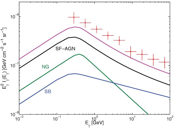 |
Figure 7. Diffuse gamma-ray emission as a function of the energy (without EBL attenuation) for the three different SFG contributions to the DGRB: quiescent SFGs (green, labeled “NG” in the figure), starburst SFGs (blue) and SFGs hosting an AGN (black). The solid pink indicates their sum. The DGRB from Ref. [8] is plotted in red. Taken from Ref. [161]. |
Pulsars are highly magnetized and rapidly spinning neutron stars, with a
beam of radiation that periodically intersects the Earth. Their initial spin
P decreases due to magnetic dipole braking
[168],
so that the time derivative of the period
 can be written as
follows
[36,
37,
169,
170,
38]:
can be written as
follows
[36,
37,
169,
170,
38]:
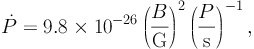 |
(11) |
where B is the surface magnetic field. The loss of kinetic energy
associated with the slowing down of the spinning, i.e. the so-called
“spin-down luminosity”
 , is
, is
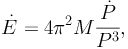 |
(12) |
where M is the moment of inertia of the neutron star. The spin-down luminosity is converted, with some efficiency, into radiation. MSPs were traditionally detected in radio, while, nowadays, thanks to the Fermi LAT, an increasingly large number of objects is observed also in the gamma-ray band. The shape of their gamma-ray energy spectra suggests that the emission comes from curvature radiation. This is a mechanism similar to synchrotron radiation, in which gamma rays are produced by relativistic charged particles following the curved force lines of a magnetic field [171, 172, 173]. Self-synchrotron Compton possibly also contributes [174].
Pulsars are classified in terms of their period and sources with
P < 15 ms
are referred to as MSPs. These are generally part of a binary system and
their higher spin is the result of the large angular momentum transferred
from the companion object
[175,
176,
177,
178,
179].
Thanks to lower surface magnetic fields, MSPs
have smaller and
are, therefore, older than “normal” (i.e., young)
pulsars. A longer life cycle may compensate the intrinsic lower
birthrate so that MSPs are expected to be as abundant as normal pulsars
[180].
Moreover, having had the time to orbit many times around the Galaxy, the
distribution of MSPs is expected to be uncorrelated with their birth
locations, potentially extending to high Galactic latitudes
[36].
The conversion of energy loss
into
Lγ is parametrized by an
empirical relation of the form
 |
(13) |
[181], where η is the called “conversion efficiency”. The case of α = 0.5 is motivated in Refs. [182, 183, 181] and adopted in Refs. [184, 37, 169], even if some of those references also consider the case of α = 1. Assuming that Eq. (13) is valid both for young pulsars and for MSPs, their luminosities are related by
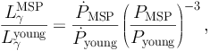 |
(14) |
for α = 1. Typical values are PMSP = 3 ms,
Pyoung = 0.5 ms,
MSP =
10−19 and
young
= 10−15. These suggest that
MSPs can be brighter than normal pulsars, by a factor of few tens. It is,
therefore, reasonable to speculate that these sources can contribute
significantly to the DGRB emission
[36,
37,
185,
169,
38].
On the other hand, the cumulative emission of normal pulsars would be
quite anisotropic and mainly localized along the Galactic plane, thus
hardly compatible with the DGRB
[186,
184].
The second Fermi LAT catalog of gamma-ray pulsars (2FPC) contains 117 sources, 40 of which are MSPs [170]. The number is too low to build a MSP LF only from Fermi LAT data. Also, given the uncertainties on the mechanisms of gamma-ray emission, it is not possible to postulate correlations with other frequencies, as done for blazars, MAGNs and SFGs. This is the reason why Refs. [36, 37, 169, 38] rely on Monte Carlo simulations in order to properly describe the population of MSPs. Probability distributions of the most relevant quantities (e.g., radial and vertical position of the source, its period and surface magnetic field) are derived from the pulsars detected in radio [187, 180, 188]. At date, the largest catalog of pulsars is the Australia Telescope National Facility Pulsar catalog, containing 1509 sources, out of which 132 are MSPs [189]. Ref. [38] analyses the objects in the catalog and establishes that they are well described by the following prescriptions: i) a Gaussian distribution for the radial distance, R, from the center of the MW projected on the Galactic plane, i.e. dN / dR ∝ exp[− (R − ⟨ R ⟩) / R0], ii) an exponential distribution for the vertical distance, z, from the Galactic plane, i.e. dN / dz ∝ exp(−z / z0) [187, 184], iii) a log-Gaussian distribution for the period P (in contrast to previous works [36, 37, 169]) and iv) a log-Gaussian distribution for the magnetic field.
Ref.
[38]
also studies the relation between Lγ and
. The data, however,
are affected by quite large errors which prevent
a statistically meaningful fit to the data. Thus, Ref.
[38]
identifies a benchmark case with α=1 that provides a qualitative good
description of the data, and an uncertainty band that encompasses
reasonably well the distribution of the data points. This completes the
characterization of the MSP population and synthetic sources can be
generated by randomly drawing from the assumed distributions. Each
source is labeled as “resolved” or
“unresolved” depending on whether its flux is larger or
smaller than the sensitivity of the telescope at the position of the
source in the sky. Simulated sources are accumulated until the number of
“resolved” ones equals the amount of detected MSPs: Refs.
[184,
37]
consider the MSPs detected in radio in the Australia
Telescope National Facility catalog
[190],
while Refs.
[169,
38]
the sources detected by the Fermi LAT.
14
This calibrates the Monte Carlo data
and it allows the computation of the MSP contribution to the DGRB simply by
summing over the “unresolved” sources. Their energy
spectrum is fixed to a power law with an exponential cut-off, i.e a
functional shape that reproduces well the MSPs in the 2FPC. The slopes
and cut-off energies are assumed to have Gaussian distributions. The
results of Ref.
[38]
are shown in Fig. 8, from which it is evident
that MSPs are only a subdominant component to the DGRB, responsible for
less than 1% of the intensity measured by the Fermi LAT in Ref.
[8].
This value is lower than the previous estimates from Refs.
[37,
169],
in which a different modeling of the MSP population was adopted.
 |
Figure 8. Prediction for the contribution of unresolved MSPs to the DGRB, as derived from 1000 Monte Carlo simulations of the MSP population of the MW. The red solid line represents the mean spectrum distribution (see Ref. [38] for further details), while the orange band corresponds to its 1σ uncertainty band. The black points refer to the preliminary DGRB measurement anticipated in Ref. [112]. Taken from Ref. [38]. |
2.2.5. Other astrophysical components
Several other potential contributors to the DGRB have been proposed in the past. Some correspond to unresolved astrophysical populations not considered in the previous sections, while others are intrinsically diffuse processes. In this section, we focus on astrophysical scenarios, while a potential DM-induced emission will be discussed in detail in Sec. 2.3.
Clusters of galaxies: it is believed that huge amounts of energy, of the order of 1061 − 1063 erg, is dissipated in the shocks associated with the assembly of clusters of galaxies [191, 192]. A fraction of this energy can go into the acceleration of CRs, even if the details of the acceleration mechanisms are still uncertain [193]. Accelerated CRs would produce gamma rays by means of i) the decay of pions produced by the interaction of CR protons with the intracluster medium and ii) IC scattering of primary CR electrons or of the electrons produced by the pion decays in point i). Yet, no gamma-ray emission has been detected from galaxy clusters. On the other hand, the interpretation of the observed radio emission as synchrotron radiation confirmed the presence of accelerated electrons and magnetic fields [194, 195]. However, not all known clusters emit in radio [196, 197] and it is not clear why some objects are radio-quiet.
The IC-induced gamma-ray emission [198, 199] depends on the abundance of CR electrons, on the intensity of the magnetic field and on the so-called acceleration efficiency ξe, i.e. the fraction of the thermal energy density produced by the shocks that is transferred to CR electrons. A Halo Model [200, 201], linking the properties of the shock to those of the DM halo hosting the cluster [202, 203], is often used to predict the IC-induced emission of clusters. Results can be tested with N-body simulations. An acceleration efficiency of ξe = 0.05 is typically assumed, following similar values measured in shocks surrounding supernova remnants. For this ξe, Ref. [202] finds that the cumulative IC-induced gamma-ray flux from unresolved clusters can explain, at most, 10% of the EGRET DGRB in Ref. [6]. Similar values are obtained by Refs. [204, 205, 206, 107, 207]. Yet, the non-detection of gamma rays from the observation of the Coma galaxy cluster suggests even lower efficiencies (ξe < 1%) [208], which would further decrease the contribution of this source class to the DGRB.
On the other hand, the gamma-ray emission expected from pion decay can be estimated as a function of the amount of gas in the intracluster medium, of the injected spectrum of CR protons and of the intensity of the magnetic fields [209]. Ref. [210] estimates that this hadronic gamma-ray emission can only account for less than few percents of the DGRB reported by EGRET in Ref. [6]. This result was later reduced to less than 1% of the Fermi LAT DGRB in Ref. [8], after that mock catalogs of clusters from Ref. [211] were considered in Ref. [208].
The most recent predictions for the emission of unresolved clusters come from Ref. [39]. In this paper, a correlation between the mass of the cluster and its gamma-ray luminosity is assumed and it is calibrated to reproduce the number of clusters detected in radio during the Radio Astronomy Observatory Very Large Array sky survey [212]. It is also required that results are compatible with the non-detection of the Coma cluster by the Fermi LAT [208] and of the Perseus cluster by MAGIC [213]. A second, more physically motivated, model for the distribution of CRs and of the intracluster medium distribution is also considered in Ref. [39]. In this case, the intracluster medium is reconstructed from X-ray observations and the CR spatial and spectral distributions are based on hydrodynamic N-body simulations [211]. The two scenarios agree in finding that the contribution of galaxy clusters to the DGRB is negligible.
Interactions of ultra-high-energy cosmic rays with background radiation: UHECRs, with energies larger than 6 × 10¹⁹ eV are attenuated due to their pion-producing interactions with the CMB, i.e. the so-called Greisen-Zatsepin-Kuzmin cut-off [214, 215]). Pions trigger electromagnetic cascades, effectively transferring energy from the CRs to the GeV-TeV energy range. This can potentially contribute to the DGRB [216, 42, 43, 217]. Ref. [42] estimates this emission, showing that it is subject to large uncertainties. Indeed, the signal strongly depends on the evolution of the UHECRs with redshift, on their composition and on the intensity of the magnetic fields encountered during the propagation of the CRs. The uncertainty on the intensity of the emission spans more than two orders of magnitude below 10 GeV. The most optimistic prediction indicates that UHECRs can indeed represent a significant contribution to the EGRET DGRB in Refs. [6, 7]. However, above 10 GeV, the intensity of the signal reduce significantly so that it would not be able to explain the bulk of the sub-TeV DGRB detected by the Fermi LAT.
Type Ia supernovae: Type
Ia supernovae are generated in the thermonuclear explosions of white
dwarfs near the Chandrasekhar mass
[218,
219].
Gamma-ray emission results from the decay of the material (mainly
56Ni) produced during the detonation. Refs.
[220,
221,
40]
compute the cumulative emission associated to this class of supernovae
as a function of their event rate. The latter is either measured
directly or related to the cosmic SFR,
⋆(z), through a model of the
delay time, i.e. the time required for a Type Ia supernova progenitor to
become a supernova. The cumulative gamma-ray emission can contribute
significantly to the DGRB only around the MeV scale (see also Ref.
[222]).
On the other hand, Ref. [41] computes the emission associated with the decay of neutral pions produced in the interactions of CR protons with the interstellar medium of the galaxy hosting the supernova. This is a scenario very similar to the one described in Sec. 2.2.3 for SFGs. However, in Ref. [41], the authors consider CRs accelerated in shocks induced by the explosions of Type Ia supernovae and not of the core-collapse supernovae, as done in Sec. 2.2.3. The predictions of Ref. [41] are affected by a significant uncertainty and they span a range between less than 10% and 100% of the DGRB reported by the Fermi LAT in Ref. [8] between 1-10 GeV.
Gamma-Ray Bursts: gamma-ray bursts are very short and intense episodes of beamed gamma-ray emission with a bimodal SED [223, 224, 225]. As in the case of AGNs, the low- and high-frequency peak are associated, respectively, with synchrotron radiation and IC. The widely-accepted fireball internal-external shock model [226] allows to describe the phenomenology of the material inside the bursts and to predict the SED of the bursts. Refs. [227, 228] estimate the total contribution of unresolved gamma-ray bursts to the DGRB by adopting the LF given in Ref. [229]. Results suggest that this emission can explain only a small fraction of the EGRET DGRB in Ref. [6], becoming negligible at energies above ∼ 40 GeV. Similar results have been obtained in Ref. [230] which estimates the contribution of unresolved gamma-ray bursts to be as large as 0.1% of the EGRET DGRB in Ref. [6] at the GeV scale.
Small Solar-system bodies: our knowledge of comets populating the Oort Cloud is quite limited and it comes almost entirely from numerical simulations. We believe that more than 1012 objects, with sizes ranging from 1 to 50 km, may populate that region. These small Solar-system bodies emit gamma rays from the hadronic interactions of CRs impinging on them. Their abundance is the main unknown, with column densities of Solar-system bodies spanning over three orders of magnitude. As a consequence, a similar level of uncertainty affects the predictions for their cumulative gamma-ray emission. Their contribution to the DGRB may go from overpredicting the DGRB measured in Ref. [7] to being responsible for only few percents of it. See Ref. [231] and references therein.
Radio-quiet AGNs: AGNs at sub-Eddington luminosities are characterized by radiatively inefficient accretions. Since the jet is not beamed enough to trigger non-thermal emission, the source emits mainly between IR and X-ray frequencies. Gamma rays can still be produced: one possibility is to have proton-proton interactions producing neutral pions in the hot gas surrounding the supermassive Black Hole. The intensity of the signal depends on the spin of the Black Hole, since more rapidly rotating objects correspond to larger X-to-gamma flux ratio [232, 233, 234]. Another possibility is a population of non-thermal electrons that can be accelerated in the hot corona around the AGN [235, 16]. The similarities between solar coronae and accretion disks [236] suggest that magnetic reconnection could be responsible for this acceleration [237]. The scenario is considered in Refs. [235, 16] where, using a luminosity-dependent-density evolution, the authors determine that this contribution can explain the whole DGRB measured by EGRET in Refs. [6, 7], but only below 1 GeV.
Imperfect knowledge of the Galactic foreground: the authors of Ref. [238] reconsidered the measurement of the DGRB by EGRET and noted that some modifications on the modeling of Galactic CRs could decrease significantly the intensity of the DGRB. They also raised some doubts on the approach of template fitting. In particular, the effect of an extended halo of electrons around the MW (with a consequent IC gamma-ray emission extending to high latitudes) is considered. Furthermore, Ref. [239] investigates the possibility of a gas cloud with a mass of few 1010 M⊙, extending to hundreds of kpc from the center of the MW. This halo would be theoretically well motivated, as it would alleviate the problem of the missing baryons in spiral galaxies. A similar object around spiral galaxy NGC 1961 would also explain the diffuse X-ray detected in Ref. [240]. Hints of such large halo could be already present in hydrodynamical N-body simulations of our Galaxy [241, 242, 239]. The gamma-ray emission associated with pion decay in this hypothetical gas halo would be able to explain between 3% and 10% of the Fermi LAT DGRB in Ref. [8], depending on the exact size of the halo.
Other possibilities not considered in the list above include emission from massive black holes at z ∼ 100 [243], from the evaporation of primordial black holes [244, 245], from the annihilations at the boundaries of cosmic matter and anti-matter domains [246] and from the decays of Higgs or gauge bosons produced from cosmic topological defects [247].
We conclude this section by discussing Fig. 9. The image gathers the most recent predictions for the “guaranteed” components to the DGRB, i.e. the emission associated with unresolved blazars, MAGNs, SFGs and MSPs (see sections from 2.2.1 to 2.2.4). They are taken from the results of Refs. [25, 29, 161, 38], respectively and they are depicted in Fig. 9 by orange, green, blue and red lines, respectively. 15 Each contribution is embedded in a band that denotes the level of uncertainty affecting the prediction. The largest is the one associated with MAGNs (light green band) spanning almost one order of magnitude. Black data points represent the new Fermi LAT measurement of the DGRB in Ref. [9] (see Sec. 2.1). The gray boxes around the data points indicate the systematic error associated with the modeling of the Galactic foreground. From the figure, it is clear that MSPs are subdominant and that the remaining 3 astrophysical components can potentially explain the whole DGRB, leaving very little room for additional contributions (see also Refs. [61, 248, 217]). Similar results have been recently obtained by Ref. [65]. This reference also shows that the goodness of the fit to the Fermi LAT DGRB energy spectrum in terms of astrophysical sources depends significantly on the model adopted for the diffuse Galactic foreground and on the slope of the energy spectrum of unresolved SFGs. In particular, a description of SFGs with a softer energy spectrum (similar to that of the Galactic foreground) can provide a better fit to the DGRB intensity.
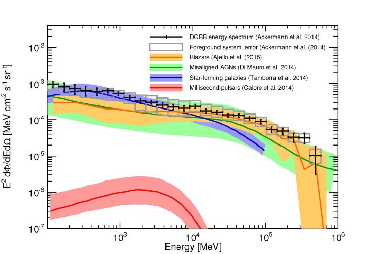 |
Figure 9. The energy spectrum of the DGRB (black points) as recently measured by the Fermi LAT [9]. Gray boxes around each data point denote the uncertainty associated with the Galactic diffuse emission. The solid color lines indicate the expected gamma-ray emission from unresolved sources, for 4 different well-established astrophysical populations: blazars (in orange), MAGNs (in green), SFGs (in blue) and MSPs (in red). Color bands represent the corresponding uncertainties on the emission of each population. Estimates are taken from Ref. [25] (blazars), Ref. [29] (MAGNs), Ref. [161] (SFGs) and Ref. [38] (MSPs). |
2.3. The Dark Matter component of the Diffuse Gamma-Ray Background
The DGRB can also be used to investigate more exotic scenarios than those presented in the above subsections. In particular, it has already been shown that the DGRB is a powerful tool to investigate the nature of DM.
Discussing the very wide range of viable DM candidates is beyond the scope of this review (see, e.g., Ref. [249]). In the following, we only consider a family of candidates called Weakly Interacting Massive Particles (WIMPs), loosely characterized by a mass of the order of the GeV-TeV and by weak-scale interactions. This is a very well studied scenario since many extensions of the Standard Model of Particle Physics predict the existence of WIMPs [250, 251, 44, 252, 253]. It is also quite natural for WIMPs to reproduce the DM relic density observed, e.g., by Planck [254]. Yet, currently there is no observational confirmation of the existence of WIMPs.
WIMP DM can either annihilate or decay into Standard Model particles, including gamma rays. This is a general prediction of WIMP candidates and it represents an additional reason to focus only on WIMPs for this review. The specific mechanisms of gamma-ray emission (see, e.g., Ref. [44] for a review) depend on the DM candidate considered and include i) direct production of monochromatic gamma rays, ii) decay of neutral pions, produced by the hadronization of the primary annihilation/decay products, iii) final state radiation and iv) secondary emission by IC or bremsstrahlung of primarily produced leptons. Since no DM source has been unambiguously detected up to now, the entire DM-induced gamma-ray emission may be unresolved and, thus, it contributes to the DGRB. In Sec. 2.3.1 we discuss the potential DM contribution to the DGRB in the case of self-annihilating DM particles, while Sec. 2.3.2 is devoted to decaying DM. Note that some DM candidates can experience both annihilations and decays [255].
DM-induced gamma rays can be produced in the DM halo of the MW or in extragalactic DM structures and substructures. We refer to the two possibilities as the “Galactic” and “cosmological” DM components, respectively. The latter is isotropic by construction, while the former is expected to exhibit some anisotropy, due to the particular location of the Earth in the DM halo of the MW. We remind that, as described in Sec. 2.1, the intensity of the DGRB is obtained by means of an isotropic template [9]. However, the Galactic DM signal can exhibit a significant anisotropy and, in that case, it cannot be considered part of the DGRB. 16 In this section, we focus mainly on the contribution of the cosmological DM signal to the DGRB, discussing a possible Galactic DM component only towards the end of the section.
2.3.1. The case of annihilating Dark Matter
In the ΛCDM cosmological framework [254], initial matter fluctuations in the Early Universe are the seeds of the structures that populate today’s Universe. These fluctuations grow by accreting new matter and form the first protostructures, which, then, collapse and eventually virialize into DM halos. ΛCDM predicts that, in later epochs, larger halos gradually assemble by accretion and merging of smaller halos. Under this scenario of structure formation, a cosmological gamma-ray signal is expected from the annihilations of DM particles taking place in all DM halos at all cosmic epochs.
The cosmological gamma-ray flux dΦ / dE0 dΩ (i.e. the number of photons per unit energy, time, area and solid angle) produced by DM annihilations at energy E0 over all redshifts z is given by [48, 49, 51]:
 |
(15) |
where mχ is the mass of the DM particle,
⟨ σ v ⟩ its annihilation cross section
17
and the sum runs over all the possible annihilation channels, each of
them corresponding to a specific branching ratio Bi
and a differential photon yield dNi / dE.
Ωχ,0 is the current DM density ratio,
c the critical density of the Universe, and
H(z) and c are the Hubble parameter and the speed
of light, respectively. The function τEBL(E,
z) accounts for the absorption of gamma-ray photons due to
interactions with the EBL. Finally, the quantity ζ(z) is
the so-called flux multiplier and it indicates
the variance of the fluctuations in the field of squared DM density. It is,
therefore, a measure of the statistical clustering of DM in the Universe:
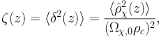 |
(16) |
where  χ is the comoving DM density and the
parentheses ⟨ · ⟩ denote angular integration over all
the possible pointings in the sky.
χ is the comoving DM density and the
parentheses ⟨ · ⟩ denote angular integration over all
the possible pointings in the sky.
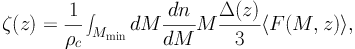
Two approaches have been proposed to calculate the flux multiplier. The first is based on the Halo Model [200, 201] and it relies on the knowledge of the abundance and of the internal properties of DM halos. The former is described by the Halo Mass Function (HMF), dn / dM, i.e. the comoving number of halos per unit mass, while the latter is encoded in the DM halo density profile. More specifically, in the Halo Model framework, ζ(z) is proportional to the integral of the HMF times the integral of the DM density squared inside the halo [48, 49, 50, 64]:
 |
(17) |
where Mmin is the minimum halo mass. Typical values for Mmin range approximately between 10−12 and 10−3 M⊙ for supersymmetric DM candidates. 18 Its exact value depends on the position of a cut-off in the power spectrum of matter fluctuations, above which the formation of DM structures is suppressed. This cut-off arises from the combined effect of kinetic decoupling and baryonic acoustic oscillations [258, 259, 260, 261], and its precise location ultimately depends on the Particle Physics nature of the DM candidate [262, 261, 263]. In addition, the mapping between the cut-off scale and Mmin is not well defined, depending on the assumed relation between mass and size of the small-mass halos [264]. These uncertainties are responsible for the huge variability of Mmin quoted above.
The factor Δ(z) in Eq. (17) is the so-called halo
overdensity and it depends on the cosmology assumed and on the details
of the gravitational collapse of the halo. The radius
RΔ at which the mean
enclosed density of a DM halo is Δ(z) times
 c is called the
virial radius, which can be taken as a measurement of the size of
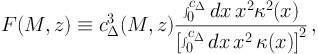
the halo. The DM distribution inside the halo is codified in the function
⟨ F (M, z)⟩:
c is called the
virial radius, which can be taken as a measurement of the size of
the halo. The DM distribution inside the halo is codified in the function
⟨ F (M, z)⟩:
 |
(18) |
where κ(x) is the DM density profile and x = r / rs. rs is a scale radius, whose precise definition depends on the assumed κ(x). The quantity cΔ is the so-called concentration [265, 266, 267] and it is defined as RΔ / rs. Note that ⟨ F (M, z) ⟩ in Eq. (17) is the function F(M, z) from Eq. (18) averaged over a log-normal probability distribution assumed for cΔ. Such a distribution accounts for halo-to-halo scatter on the value of cΔ [265, 268, 269], which is a natural consequence of the stochastic process of structure formation in ΛCDM cosmology.
Information on the abundance and internal properties of DM halos is mainly extracted from N-body cosmological simulations (see, e.g., Ref. [270] and references therein). However, simulations do not resolve the whole halo hierarchy down to Mmin. The current resolution limit for MW-like DM halos is approximately at 105 M⊙ at z = 0 [271], i.e. several orders of magnitude above the expected value for Mmin. Thus, extrapolations of the relevant quantities (e.g., the HMF and cΔ(M, z)) are needed. Since F(M, z) in Eq. (18) depends on the third power of the halo concentration, the way cΔ(M, z) is extended below the mass resolution of simulations is crucial in the estimation of the cosmological DM signal. Above the mass resolution limit, cΔ(M) can be well described by a power law [265, 272, 273, 266, 267]. Several works assume the same behavior to be valid down to Mmin [274, 56, 275, 276], thus assigning very large concentrations to the smallest halos. This translates into a very high gamma-ray flux expected from DM annihilations. Nevertheless, power-law extrapolations for cΔ(M) are not physically motivated and they are now clearly ruled out both by recent high-resolution simulations of the smallest DM halos [277, 278, 279] and by theoretical predictions deeply rooted in the ΛCDM cosmological framework [267, 280, 281]. Indeed, simulation-based and theoretical estimates of cΔ(M, z) have been shown to agree now remarkably well over the full halo mass range, i.e. from Earth-like “microhalos” up to the scale of the heaviest galaxy clusters [280]. Compared to power-law extrapolations, these estimates exhibit a flattening of cΔ(M) at low masses. This leads to substantially less concentrated low-mass halos and, thus, to a considerably smaller cosmological DM signal. Overall, predictions for the cosmological DM-induced emission can vary by few orders of magnitude depending on the adopted model for cΔ(M, z) in Eq. (18), see, e.g., Refs. [56, 282].
Not unexpectedly, the variability of the predicted DM signal also depend on the particular choice of Mmin. For example, the cosmological signal increases by up to a factor of ∼ 6 when Mmin goes from 10−3 M⊙ / h to 10−12 M⊙ / h [62]. This refers to the case of a power-law extrapolation of cΔ(M) and, by construction, flux multipliers that rely on power-law extrapolations are particularly sensitive to the choice of Mmin. When adopting a cΔ(M) that flattens at low halo masses, the flux multiplier changes by a factor of ∼ 3 over the same range of Mmin [62, 64].
N-body cosmological simulations have also been employed to understand the HMF and its redshift evolution [283, 284]. Mock halo catalogs have been used to test the predictions of the Press-Schechter formalism, according to which the HMF can be written as follows [200, 285, 286, 287]:
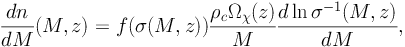 |
(19) |
where σ(M, z) is the variance of the fluctuations of the DM density field (smoothed on a scale of mass M) and the exact expression for f(x) depends on the mechanism assumed to describe the halo gravitational collapse. An accurate fitting formula for the HMF, inspired by Ref. [288], can be found in Ref. [289] for the cosmological model favored by the first data release of the Wilkinson Microwave Anisotropy Probe (WMAP). More recently, Ref. [267] have also adopted the functional form proposed in Ref. [289] and derived the parameters of the HMF compatible with the cosmological model preferred by Planck. 19 Overall, the HMF at z = 0 can be qualitatively approximated by a power law with a slope between -1.9 and -2.0 and a sharp cut-off for halos more massive than ∼ 1014 M⊙. The uncertainty in the calculation of the cosmological DM signal induced by different possible parametrizations of the HMF is only marginal when compared to other sources of uncertainties. For instance, assuming the HMF of Ref. [288] instead of the one in Ref. [289] changes the total gamma-ray flux by a factor of about 20% (see also Ref. [282]).
High-resolution N-body simulations have also helped to establish the density profiles of DM halos in great detail. Ref. [291] determined that DM halos exhibit a density profile that is universal, i.e. independent of the halo mass. A Navarro-Frenk-White (NFW) profile, i.e. proportional to κ ∝ 1 / r in the inner region and to a steeper r−3 at large radii, provides a good fit. More recently, the so-called Einasto profile was found to agree better with the results of N-body simulations, especially at intermediate halo radii [292, 293, 294]. Even if many other parametrizations have been proposed over the last years [295, 296, 297, 298, 299, 300], current N-body simulations agree on a slope ≲ −1 for the DM density in the inner region. However, these “cuspy” profiles are derived from simulations that only contain DM, without including baryons. Indeed, high-resolution observations of the rotation curves of DM-dominated dwarfs and low-surface-brightness galaxies favor DM density profiles with a flat central core [301, 302, 303, 304, 305, 306, 307, 308, 309]. Phenomenological cored profiles, such as the Burkert one [302], were proposed to accommodate such results. More recently, hydrodynamical simulations have been performed, which realistically include the complexity of baryonic physics. They begin to reproduce the observed properties of galaxies successfully, e.g. in Refs. [310, 311]. Yet, the exact interplay between baryons and DM at all radial scales and for all halo masses is not fully understood, and the impact of complex baryonic phenomena (such as supernova feedback, stellar winds and baryonic adiabatic compression) on the DM density profile is still uncertain, particularly in the inner region [312, 313, 314, 315, 316, 317, 318, 319, 320]. Ref. [321] finds a difference of almost one order of magnitude in the cosmological flux when a Burkert profile is assumed for all DM halos instead of a NFW one.
In addition to DM halos, a natural prediction of ΛCDM is the existence of a large number of subhalos, i.e. halos gravitationally bound to a larger host halo and located within its virial radius. Since the annihilation luminosity of a halo is proportional to its DM density squared, the presence of small clumps with high DM densities has the effect of boosting the overall gamma-ray luminosity of the host halo [322, 323, 324, 274, 325, 326, 327, 56, 328, 329, 275, 330, 276, 279, 331, 280]. The additional contribution from substructures can be accounted for in the computation of the flux multiplier by adding an extra term in Eq. (17). In particular, the factor ⟨ F(M, z) ⟩ has to be replaced by ⟨ F(M, z) ⟩ (1 + B(M, z)), where B(M, z) is called the “boost factor”. 20
The subhalo population is characterized by a subhalo mass function:
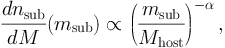 |
(20) |
extending down to Mmin. The slope of the subhalo mass function has been measured in high-resolution N-body simulations, ranging between -1.9 and -2 [323, 271]. These values are also in line with theoretical expectations from the Press-Schechter theory of structure formation [333, 334, 335]. It has been noted, though, that several effects may prevent the subhalo mass function to reach the lowest subhalo masses, since processes such as tidal disruption, accretion or merging may be particularly efficient and deplete the low-mass tail of the mass function. It is difficult to estimate the survival probability of these small subhalos, while it remains computationally very expensive to simulate and keep track of such processes with the resolution needed. Although the properties of low-mass DM subhalos are expected to follow those of the more massive counterparts, the abundance and distribution of DM substructures below the resolution of current simulations remain uncertain. The internal properties of subhalos are also subject to debate. We still lack a comprehensive understanding of the subhalo concentration, even if subhalos have been shown to exhibit larger cΔ(M) than halos of the same mass [336, 271, 337, 338]. Similarly to the case of main halos, the assumptions made on cΔ(M) and on the abundance of low-mass subhalos have a large impact on the amplitude of the subhalo boost factor. Overall, under the most extreme scenarios (corresponding to blind power-law extrapolations of cΔ(M)), the presence of subhalos can increase the total cosmological annihilation signal by more than one order of magnitude [48, 62, 217, 339].
As an alternative to the Halo Model described above, the Power Spectrum approach has been recently introduced to compute the flux multiplier [340, 264]. In this new framework, ζ(z) can be calculated by means of the non-linear matter power spectrum PNL, i.e. the Fourier transform of the two-point correlation function of the matter density field, as follows:
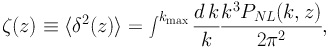 |
(21) |
where kmax(z) is a maximal scale that can be related to Mmin in the Halo Model formalism. 21 The main benefit of the Power Spectrum approach relies on the fact that only one single quantity is needed for the calculation of ζ(z), i.e. PNL in Eq. (21). PNL can be measured directly in N-body cosmological simulations using only a matter density map and it does not rely on the concept of DM halos. It is, thus, also independent on the complex issue of halo finding and on the uncertainties associated with it [341]. 22 This is, indeed, what the authors of Ref. [264] did, guided by the results of the Millennium-I and Millennium-II simulations [284, 343]. Yet, as in the Halo Model approach, current N-body simulations do not reach the highest k values needed in Eq. (21) and, thus, extrapolations beyond the simulation resolution are again required. 23 Note, however, that only PNL is extrapolated in this case, as opposed to the Halo Model approach that relies on the knowledge of several quantities in the low-mass regime. This is indeed the reason why the authors in Ref. [64] adopted the Power Spectrum approach to obtain a realistic estimate of the uncertainty on ζ(z), even if their fiducial flux multiplier is computed within the Halo Model framework. Furthermore, within the PS approach, it is possible to motivate in a realistic way both the choice of kmax and the way the extrapolation is performed. Note also that, by construction, the Power Spectrum approach naturally includes the contribution of substructures down to length scales ∼ π / kmax, while in the Halo Model the description of substructures requires additional knowledge, often leading to further debatable extrapolations and uncertainties. 24
A comparison between the Power Spectrum and Halo Model approaches is performed in Refs. [264, 344, 64]. Results from Refs. [264, 64] are reproduced in Fig. 10. In the left panel, the red bands indicate the predictions for ζ(z) (multiplied by factors depending on redshift) obtained by means of the Power Spectrum method for different choices of kmax. For each value of kmax adopted, the corresponding band accounts for different ways of extrapolating PNL beyond the resolution of the Millennium simulations. The predictions for the Halo Model (gray band) refer to a Mmin = 10−6 M⊙ / h and have been obtained following Refs. [56, 58]. In the right panel of Fig. 10, the predictions of the Power Spectrum approach (for a specific value of kmax) are given by the gray band. The width of the band corresponds to two different prescriptions to perform the extrapolation (labeled “PS (min)” and “PS (max)” in the figure). On the other hand, the red band reproduces the results of the Halo Model in Ref. [64] for Mmin = 10−6 M⊙ / h and two values of the slope for the subhalo mass function. Remarkably, the two methods agree well in their predictions for ζ(z), within uncertainties. This is so despite the caveats mentioned above and the intrinsic differences of the two formalisms.
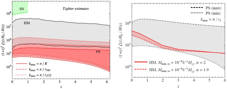 |
Figure 10. Comparison of the Halo Model and Power Spectrum approaches for the calculation of the flux multiplier. The Halo Model makes use of Eq. (18) while the Power Spectrum formalisms adopts Eq. (21). Left: Power Spectrum predictions are shown in red. The different bands correspond to different prescriptions to derive the cut-off scale kmax from the size of the DM halo with mass Mmin. The width of the bands accounts for different extrapolation schemes up to kmax. The Halo Model predictions (gray band) are obtained following Refs. [56] and [58]. Figure taken from Ref. [264]. Right: Predictions according to the Power Spectrum approach (gray) and the Halo Model (red). The Halo Model formalism follows what done in Ref. [64] for two possible subhalo mass functions. The gray band corresponds to a particular choice of kmax in the Power Spectrum approach, for different ways (labeled as “PS (max)” and “PS (min)” in the figure) to extend PNL beyond the resolution of the simulations. For both panels, a value of Mmin = 10−6M⊙ / h is adopted in the Halo Model formalism. Figure taken from Ref. [64]. |
From Sec. 2.2 we know that gamma-ray emission of astrophysical origin is able to explain a significant fraction, if not all, of the DGRB, therefore leaving very little room for a potential DM contribution (see also Fig. 9). Moreover, the gamma-ray energy spectrum expected from DM annihilations is generally slightly curved, with a cut-off at the mass of the DM particle and the possibility of spectral features like bumps or lines. On the other hand, the DGRB detected by the Fermi LAT exhibits a power-law spectrum at low energies and a cut-off compatible with EBL attenuation at higher energies (see Sec. 2.1). This suggests, again, that DM annihilations cannot provide a dominant contribution to the DGRB. Thus, the DGRB can be used to set limits on the intensity of the DM-induced emission. These are usually translated into upper limits in the (mχ,⟨ σ v ⟩) plane, identifying the region that, given a model for the abundance and properties of DM halos and subhalos, is excluded as it overproduces the measured DGRB.
Most of the works following this idea employ the Halo Model approach to predict the cosmological DM annihilation signal. Given the large number of parameters involved in the Halo Model framework, as well as the large uncertainties associated with some of them, it is very hard to perform a detailed, one-to-one comparison among the different DM limits available in the literature. In particular, predictions obtained by different groups differ mainly due to different assumptions on cΔ(M, z) and Mmin. In addition, some works also consider the Galactic DM signal. Differences can be further amplified by the various statistical prescriptions employed to compute the upper limits. Yet, we believe that a comparison among the limits in the literature is useful, as it showcases the potential of searching for DM in the DGRB compared to other indirect DM probes. Fig. 11 summarizes some of the upper limits available. 25 They all refer to annihilations entirely into b quarks. Note that the limits obtained by assuming a power-law cΔ(M) below the mass resolution of N-body simulations are among the most constraining in Fig. 11 (see, e.g., the gray dashed line from Ref. [217]). However, as argued above, power-law cΔ(M) are not well motivated, putting the corresponding limits into question.
 |
Figure 11. Upper limits obtained by considering the DGRB energy spectrum measured in Refs. [8, 9]. Annihilations into b quarks are assumed. The regions above the colored lines are excluded because the cumulative DM-induced emission would overproduce the DGRB. Different lines correspond to different assumptions for the properties of DM halos (especially for low halo masses) and different methods to compute the upper limits. The solid green line is taken from Fig. 2 of Ref. [365] while the dashed green line is from Fig. 8 of Ref. [335] (lower bound of the band relative to αm = 2 for the emission from the Galactic Poles). The dashed blue line is taken from Fig. 5 of Ref. [58] (conservative limits for model MSII-Sub1) and the solid gray one from Fig. 2 of Ref. [367]. The solid and dashed red lines are taken from Fig. 3 of Ref. [61] (limits labeled “Fermi EGB”) and from Fig. 5 of Ref. [248] (panel labeled “best-fit background”), respectively. The dashed gray line is from Fig. 15 of Ref. [217] (default substructures’ model). The black lines correspond to the predictions obtained in Ref. [64] by means of the Halo Model (reference scenario). The solid blue line is taken from Fig. 4 of Ref. [25], while the dashed purple one is from Fig. 4 of Ref. [65]. The blue region indicates the portion of the (mχ,⟨ σ v ⟩) plane already excluded by the observation of the Segue 1 dwarf Spheroidal galaxy performed by the MAGIC telescopes (see Fig. 6 of Ref. [368]). The dark gray region is excluded by the analysis performed by the H.E.S.S. telescopes in Ref. [369] from the so-called “Galactic Center halo” (see their Fig. 4 for an Einasto DM density profile). Finally, the light gray region indicates the DM candidates not compatible with the combined analysis of 15 dwarf Spheroidal galaxies by the Fermi LAT [370]. A comparison between the Fermi LAT DGRB and the DM-induced signal can also be found in Refs. [366, 59, 60, 109, 62, 339]. The dash-dotted horizontal line marks the value of the thermally averaged annihilation cross section. |
Two approaches are possible when deriving DM limits from the DGRB measurement. In the first one it is required that the DM signal does not overshoot the measured DGRB at a particular confidence level, typically 2 or 3σ. See, e.g., Refs. [365, 59, 366, 60, 62, 335, 339]. This leads to conservative and robust upper limits on the DM annihilation cross section, shown by the green lines in Fig. 11. Alternatively, one or more astrophysical contributions to the DGRB can be modeled and included in the analysis. The DM component is, then, required not to overshoot the fraction of the DGRB not already accounted for by astrophysics. These limits are more constraining than the previous ones [58, 367, 61, 109, 248, 217]. Nevertheless, since the exact contribution from astrophysical sources is not known, it must be noted that they are subject to larger uncertainties.
The most recent constraints on annihilating DM comes from Ref.
[64]
and are shown by black lines in
Fig. 11. The “conservative limit”
(solid black line) is obtained without including any modeling of
astrophysical contributors to the DGRB. These limits exclude
annihilation cross sections a factor of ∼ 3 lower than the
thermal value of 3 × 10⁻²⁶ cm3
s−1 for a mass of 10 GeV, while, for
mχ ≥ 1 TeV, the upper limit is around
5 × 10⁻²⁴ cm3
s−1. Ref.
[64]
also shows that an improvement of one order of magnitude (a factor
∼ 2) for DM masses of the GeV scale (around 30 TeV) is possible
when i) the cumulative astrophysical contribution to the DGRB is
modeled as a power-law in energy with an exponential cut-off and
ii) slope and position of the cut-off are fixed to the best-fit
values to the DGRB data in Ref.
[9].
Note that this approach (referred to as
“sensitivity reach” and denoted by the dashed black line in
Fig. 11) does not account for any uncertainty in
the description of the astrophysical emission. A more realistic scenario is
the one of Ref.
[25],
where the authors estimate the unresolved astrophysical emitters using
the most up-to-date information from resolved sources or from other
frequencies (see Sec. 2.2). A renormalization factor
 is included
in front of the total astrophysical contribution to account for possible
fluctuations in its intensity. The limit of ⟨ σ v
⟩ (solid blue line in Fig. 11) is then
obtained by profiling over .
This results in an improvement of a factor of ∼ 3 for
mχ = 10 GeV, with respect to the conservative
limits of Ref.
[64].
A negligible improvement is expected at masses
larger than 10 TeV, where the limits are determined by the Galactic DM
signal.
is included
in front of the total astrophysical contribution to account for possible
fluctuations in its intensity. The limit of ⟨ σ v
⟩ (solid blue line in Fig. 11) is then
obtained by profiling over .
This results in an improvement of a factor of ∼ 3 for
mχ = 10 GeV, with respect to the conservative
limits of Ref.
[64].
A negligible improvement is expected at masses
larger than 10 TeV, where the limits are determined by the Galactic DM
signal.
Similar results have recently been obtained in Ref. [65], which also employs a model for the astrophysical components to the DGRB. The different statistical analysis performed in Ref. [65] suggests that a description of the DGRB of Ref. [9] in terms of unresolved astrophysical sources and gamma rays from DM annihilations in the MW halo provides a better fit, compared to a purely astrophysical interpretation with no DM. Such a hint of a DM signal in the DGRB suggests a DM particle with a mass of ∼ 10−20 GeV (for annihilation into b quarks), depending on the model adopted for the diffuse Galactic foreground. 26
Indeed, some of the limits shown in Fig. 11 have been obtained assuming that DM annihilations in the MW halo also contribute to the DGRB [58, 365, 367, 59, 366, 61, 109, 62, 335, 339, 248, 217]. Note that, as mentioned in Sec. 2.1, the DGRB is obtained from the normalization of the isotropic template in the multi-component fit to the gamma-ray data at high Galactic latitudes. Thus, when a Galactic DM signal is included, it is implicitly assumed that the DM signal is sufficiently isotropic in this particular region of the sky.
Two distinct components contribute to the Galactic DM signal. The first accounts for the smooth DM distribution of the host DM halo of the MW, while the second one comes from the population of Galactic subhalos. The former depends on the DM density profile assumed for the MW main halo. This is uncertain in the innermost parts of the Galaxy, but for |b| > 20°, i.e. more than 3 kpc from the Galactic Center, N-body simulations roughly agree. The signal from this smooth component peaks towards the Galactic Center and, between b = 20° and 90°, typical variations are of a factor of ∼ 16 [64]. Thus, even outside the Galactic plane the signal is largely anisotropic and, therefore, this component cannot be described by an isotropic template as the DGRB. Indeed, the presence of an emission with such a well-defined morphology may impact the procedure used in Ref. [9] to measure the DGRB energy spectrum. This was tested in Ref. [64], where the authors re-derived the DGRB including an additional template for the smooth Galactic DM signal. They found that this signal can be degenerate with other diffuse Galactic emissions, especially the one from IC. They also checked the impact that the new template would have on the upper limits on ⟨ σ v ⟩. The result suggests that, at least for DM candidates not excluded by the conservative limits in Ref. [64], this additional Galactic DM template has only a moderate effect.
The second contribution to the Galactic DM signal comes from the subhalos of the MW: the brightest or closest of them may potentially give rise to bright spots in the gamma-ray sky. However, none of the unassociated sources in the 2FGL catalog has been robustly interpreted as a DM subhalo [371, 372]. The overall subhalo population is expected to give rise to a diffuse smooth emission [274, 53, 55, 359]. Its morphology depends on the abundance and distribution of subhalos in the Galaxy. A general prediction is that the cumulative emission of subhalos is more extended (thus more isotropic) than that of the main halo. More specifically, factors between 0.1 and 2 are quoted in Ref. [64] for the variation of the signal of Galactic substructures between b = 20° and 90°. These small variations motivate the authors of Ref. [64] to assume this component as isotropic and, thus, to include it when setting their DM limits. Its impact can be quite significant since Galactic subhalos can boost the Galactic DM signal by a factor of 3 to 15, depending on the slope of the subhalo mass function [280].
We end this section by comparing the upper limits on the annihilation cross section derived in Ref. [64] to the results of other indirect searches for DM. In particular, in Fig. 11, the shaded regions indicate which portion of the parameter space has been already excluded by these other probes. The blue region is derived from the observation of the Segue 1 dwarf Spheroidal galaxy by the MAGIC telescopes [368], while the dark gray region indicates the portion of the (mχ,⟨ σ v ⟩) space not compatible with the analysis of H.E.S.S. data from the so-called “Galactic Center halo” [369]. Finally, the light gray area is excluded by the non-detection of gamma rays from the observation of 15 dwarf Spheroidal galaxies with the Fermi LAT [370]. Note that the conservative upper limits derived in Ref. [64] (solid black line) are always inside the area already excluded, while the most stringent sensitivity reach (dashed black line) provides the strongest constraints on ⟨ σ v ⟩ for DM masses up to 1 TeV, above which the limit from H.E.S.S. becomes more stringent.
2.3.2. The case of decaying Dark Matter
Decaying particles can be a viable DM candidates if their decay lifetime is larger than the age of the Universe [373, 374, 375]. As in the previous section, we will not discuss here the models that can accommodate such particles or the mechanisms that guarantee long lifetimes. We simply consider generic WIMPs that decay emitting gamma-ray photons.
In contrast to the case of annihilating DM, the gamma-ray signal expected from decaying DM particles is linearly proportional to the DM density. For instance, the contribution of the MW halo (at a certain energy E0 and towards the direction ψ) can be written as follows:
 |
(22) |
where τ is the DM particle lifetime,
MW the DM density profile
of the MW halo and s is the line-of-sight variable pointing
towards the direction of observation. In the case of prompt emission,
the s-wave annihilation of 2 non-relativistic DM particles with a
mass mχ is equivalent to the decay of a
s-wave state with mass 2mχ and integer spin
[376].
Under those assumptions, the photon yield dNi / dE
in Eq. (22) can be determined from the same quantity in
Eq. (15). A decaying DM candidate can also produce
gamma rays through semileptonic channels (provided that it is characterized
by a semi-integer spin) or through a three-body decays
[255].
Mono-chromatic lines are also a typical signature
of a vast class of decaying DM candidates
[377,
378,
379,
374,
380],
while the so-called “box-shaped” spectra have been
recently introduced in Ref.
[381].
Finally, secondary gamma rays can also be produced
when primary leptons from DM decay interact via bremsstrahlung with the
interstellar medium of the Galaxy or via IC off its radiation fields
[382].
Given the linear dependence on the DM density in Eq. (22), the gamma-ray signal expected from the smooth MW DM halo has a different morphology, compared to the case of annihilating DM. For a decaying particle, the emission is now more isotropic and, thus, there exists a better motivation to include it among the contributors to the DGRB. Note also that, on the case of decaying DM, the emission of a DM halo is proportional to the its total mass. This means that DM substructures are not expected to boost significantly the predicted DM signal. Therefore, for a specific DM candidate, the main uncertainty affecting the emission in Eq. (22) comes from the unknown DM density profile of the MW halo. 27 Remarkably, this translates into a considerably smaller uncertainty on the intensity of the DM-induced emission compared to the case of annihilating DM.
The cosmological signal for a decaying DM candidate is written as follows:
 |
(23) |
There is no need of including the flux multiplier since the average emission depends on the total amount of DM, accounted for by ΩDM. This eliminates any dependence on Mmin or on the shape of cΔ(M, z) and it translates into more robust predictions. 28
Many works have used the DGRB to derive constraints on the nature of decaying DM candidates. Refs. [390, 391, 392, 377, 378, 393, 394, 374] consider the DGRB measured by EGRET in Refs. [6, 7], while Refs. [386, 385, 383, 380, 59, 367, 387] rely on the DGRB measurements by the Fermi LAT. Results are summarized in Fig. 12, which collects lower limits on τ as a function of mχ. The regions below the lines in Fig. 12 are excluded since the corresponding DM particle (for a specific decay channel) produces a gamma-ray emission which is not compatible with the DGRB data. The scatter among the different lines in the figure is due both to the different statistical techniques used to derive the limits and to the different modeling adopted for the DM-induced emission. It should be noted that all lines are obtained by assuming that the DM-induced emission is the only component of the DGRB. The only exceptions are the dashed gray line from Refs. [386] and the dashed blue one from Ref. [387], in which the authors also model the astrophysical component of the DGRB. Both the Galactic and cosmological signals are considered when deriving all lower limits in Fig. 12, but the ones given by the solid gray and dashed blue lines, which correspond to Ref. [384] and Ref. [387], respectively. In these two cases, limits refer to the cosmological DM component only. Other predictions for the contribution of decaying DM to the DGRB can be found in Refs. [395, 396, 62, 397].
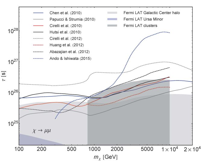 |
Figure 12. Lower limits obtained by considering the DGRB energy spectrum measured in Ref. [8]. Decays into µ+µ− are assumed. The regions below the colored lines are excluded because the cumulative DM-induced emission would overproduce the DGRB. Different lines correspond to different assumptions for the properties of DM halos and different methods to compute the lower limits. The solid blue line is taken from Fig. 3 of Ref. [383], while the solid gray one is from Fig. 8 of Ref. [384] (NFW DM density profile). The solid red and solid black lines are taken from Fig. 4 of Ref. [385] and from Fig. 6 of Ref. [59] (NFW DM density profile), respectively. The dashed gray line is from Fig. 2 of Ref. [386] (DM signal and power-law background) and the dashed red one from Fig. 4 of Ref. [380]. The dashed black line is taken from Fig. 4 of Ref. [367]. The dashed blue line comes from Fig. 3 of Ref. [387] (for model A of the Galactic foreground). The blue region indicates the portion of the (mχ, τ) plane already excluded by the observation of the Ursa Minor dwarf Spheroidal galaxy performed by the Fermi LAT (see Fig. 3 of Ref. [388], for the case of no IC emission). The dark gray region is excluded by the analysis performed in Ref. [380] combining Fermi LAT data from the position of 8 galaxy clusters (see their Fig. 4). Finally, the light gray region indicates the DM candidates not compatible with the observation of the so-called “Galactic Center halo” performed by the Fermi LAT in Ref. [389] (see their Fig. 5 for a NFW DM density profile). |
The most constraining lower limit in Fig. 12 comes from Ref. [386] (dashed gray line) below ∼ 2 TeV, and from Ref. [387] (dashed blue line) for larger DM masses. Decay lifetimes as large as 2 × 1026 s are excluded for DM masses below ∼ 500 GeV, while the limit goes up to 1028 s for mχ ∼ 10 TeV. Note that the results of Ref. [387] are obtained from the most recent Fermi LAT measurement of the DGRB reported in Ref. [9]. The authors also shows how the lower limit changes depending on the model employed to describe the diffuse Galactic foreground. Furthermore, the lower limit at large DM masses is found to vary by up to a factor of a few for different ways of parametrizing the astrophysical component of the DGRB and its uncertainty.
Compared to the limits derived from other DM targets, the dashed gray and dashed blue lines in Fig. 12 represent the most constraining information available on τ. In particular, in Fig. 12 we show the regions excluded by three different analyses performed with Fermi LAT data, namely the observation of i) the Segue 1 dwarf Spheroidal galaxy [388] (blue region), ii) 8 galaxy clusters [380] (in dark gray) and iii) the “Galactic Center halo” [389] (in light gray).
3 These values refer to the 68% containment radius. Back
4 However, note that, in the re-analysis of Ref. [81], the energy spectrum is well described by a single power law only up to 2 GeV. Back
5 A CR propagation code available from http://galprop.stanford.edu. See also Ref. [79]. Back
6 Normally S is the gamma-ray flux above some energy Emin and, therefore, it is related to FE0(z, Y, Γ) as S = ∫Emin FE0(z, Y, Γ) dE0. Back
7 More precisely, the assumed proportionality is between LX and the so-called “bolometric luminosity”, i.e. a measure of the total emission power of the source. However, under the hypothesis of the blazar sequence, Lγ can be uniquely derived from the bolometric luminosity. Back
8 The best-fit point obtained in Ref. [19] favors a γ1 much larger than the one found in Ref. [16] for EGRET blazars. Back
9 In Ref. [22] only sources with Lγ ≥ 1044 erg s−1 are considered when computing the emission of unresolved FSRQs. Such a value corresponds approximately to the fainter blazar in the 1FGL. Thus, the quoted contribution of FSRQs to the DGRB implicitly assumes that no sources are present below 1044 erg s−1 and, therefore, it should be considered as a lower limit to the total emission of unresolved FSRQs. Back
10 The luminosity functions in Ref. [29] are defined per units of log(L), hence the factor log10(Lr,i) / log10(Lγ) in Eq. (5) as compared to Eq. (4). Back
11 As done for MAGNs, gamma-ray and IR LF are defined here per unit of log(Lγ) and of log(LIR), respectively. Back
12 We note that, even if these SFGs host an AGN, their IR luminosities are expected to be dominated by the star-forming activity rather than the one associated with the AGN and, therefore, LIR remains a useful tracer of the SFR. Back
13 The low-energy slope is fixed to -1.5 in all cases, while the high-energy one is assumed to be -2.7 for quiescent galaxies and -2.2 for starburst ones. The class of AGN-hosting objects is additionally split into “starburst-like” and “quiescent-like” galaxies, with slopes of -2.2 and -2.7, respectively. Back
14 In this case the sensitivity of the Fermi LAT is taken from Ref. [170]. Back
15 Ref. [25] only provides the total emission from resolved and unresolved blazars. Since we are interested in the unresolved component, the orange line in Fig. 9 is obtained by subtracting the emission of resolved sources from Ref. [9] from the total signal from blazars. The width of the light orange band is, then, computed summing the estimated errors of the two components in quadrature. Also, the abrupt end of the SFG component at ∼ 100 GeV in not physical and simply comes from the lack of predictions above this enegy in Ref. [161] only up to that energy. Back
16 Small-scale anisotropies in the DGRB, on the other hand, are discussed in detail in Sec. 3. Back
17 The annihilation cross section in Eq. (15) is assumed to be dominated by s-wave interactions. In the case of a dependence on the relative velocity of the annihilating DM particles, Eq. (15) has to be modified accordingly and the signal will, thus, depend on the velocity distribution of DM [256, 257]. Back
18 The value Mmin = 10−6 M⊙ has become a standard benchmark value in the field. Back
19 Note that the agreement of different fitting formulas with the simulations may depend on the algorithm used by the simulators to extract the mass of a halo from the raw particle data, with the caveat that different algorithms may lead to different results [290]. Back
20 This definition of the boost factor is particularly convenient for the computation of the flux multiplier and of the cosmological DM signal. We warn the reader, though, that alternative definitions of B(M, z) can be found in the literature. Back
21 The exact relation between kmax and Mmin is not trivial, as discussed in detail in Refs. [264, 64]. Back
22 In Refs. [342, 331], the authors introduce the concept of particle phase space average density, an estimate of the coarse-grained phase-space density of DM structures. Interestingly, they show in Ref. [331] how this observable can be used to determine the DM-induced emission of MW-like halos. The particle phase space average density can be directly computed directly from N-body simulations’ raw data and, therefore, the formalism shares some similarities with the Power Spectrum approach, introduced here to estimate the cosmological DM signal. Back
23 At redshift zero, for instance, the maximum k values resolved in current large-scale structure simulations are typically of the order of few hundreds, while kmax may take values up to 106. Back
24 We remind the reader that Eq. (21) only determines the cosmological DM signal. Any gamma-ray emission associated with the halo of the MW and its subhalos is not accounted for by the Power Spectrum model and, thus, needs to be added by hand (see further discussion at the end of this section). Back
25 We only consider limits derived from the two measurements of the DGRB performed by the Fermi LAT [8, 9]. Older works based on earlier DGRB measurements can be found, e.g., in Refs. [345, 346, 347, 48, 49, 348, 349, 350, 50, 351, 51, 52, 352, 353, 354, 355, 356, 274, 357, 358, 55, 359, 321, 360, 361, 362, 363, 56, 364]. Back
26 A similar indication of a DM component to the DGRB was also reported in Refs. [348, 357] based on the EGRET measurement of the DGRB in Ref. [7]. Back
27 When considering secondary emission, one should also add the uncertainty associated with our imperfect knowledge of the propagation of charged particles in the MW [382]. Back
28 Even if one rewrites Eq. (23) in terms of the Halo Model formalism, the result of integrating the HMF times the number of gamma rays expected from a DM halo of mass M will be quite insensitive to the value adopted for Mmin [62]. Back