4.2 Single-Sample Goodness-of-Fit Tests

We set out in this section to consider comparison of samples, perhaps not the ideal way of conducting research, but necessary, for the following reasons. For single-sample comparison, i.e. comparison between one specific sample and a model or a sample of infinite size, we might wish to determine if there is a difference in location (e.g. mean) or dispersion (e.g. spread) in comparison to the known population. [The best-known parametric tests for sample comparison concern samples drawn from Normally-distributed parent populations; these tests are of course the ``Student''s' t-test (comparison of means) and the F-test (comparison of variances), and are discussed in most books on statistics, e.g. Martin 1971, Stuart & Ord 1994.] Is there a difference between observed and theoretical frequencies, i.e. between sample and model? Is the sample random from a known population?

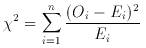
Chi-square test. We have discussed this technique in some detail in the context of model fitting via minimum ². H₀ is that the proportion of objects in each bin is as ``expected'' (from a model or from the presumed population). The procedure is to place the sample data into n bins and to compute the ² statistic, which is

for (n - 1) degrees of freedom. Once this is calculated Table A III may be consulted to determine the significance level. If consultation of Table A III shows that ² exceeds a (pre-determined) critical value for the appropriate number of degrees of freedom, H₀ is rejected at that level of significance.

To reiterate, the advantages of the test are its general acceptance, its ease of computation, the ease of guessing significance and the fact that model testing is free: vary the model parameters to turn testing to fitting as described above. The disadvantages are the loss of power and information via binning, and the lack of applicability to small samples: beware of the dreaded instability at < 5 counts per bin. Moreover, the ² test cannot tell direction, i.e. It is a ``two-tailed'' test: it can only tell whether the differences between sample and prediction exceed those that can be reasonably expected on the basis of statistical fluctuations due to the finite sample size. There must be something better, and indeed there is.

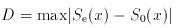
Kolmogorov-Smirnov one-sample test. The test is extremely simple to carry out.

1. Calculate S_e (x), the predicted cumulative (integral) frequency distribution under H₀.

2. Consider the sample of N observations, and compute S₀ (x), the observed cumulative distribution, the sum of all observations to each x divided by the sum of all N observations.

3. Find

   

4. Consult the known sampling distribution for D under H₀, as given in Table A IV, to determine the fate of H₀. If D exceeds a critical value at the appropriate N, then H₀ is rejected at that level of significance.

Thus as for the ² test, the sampling distribution indicates whether or not a divergence of the observed magnitude is ``reasonable'' if the difference between observations and prediction is due solely to statistical fluctuations.

The Kolmogorov-Smirnov test has some enormous advantages over the ² test. First, it treats the individual observations separately, and no information is lost because of grouping. Secondly, it works for small samples; for very small samples it is the only alternative. For intermediate sample sizes it is more powerful. Finally, note that as described here, the Kolmogorov-Smirnov test is non-directional or two-tailed, as is the ² test. However, a method of finding probabilities for the one-tailed test does exist (Birnbaum & Tingey 1951; Goodman 1954), giving the Kolmogorov-Smirnov test yet another advantage over the ² test.

Then why not always use it? There are perhaps two valid reasons, in addition to the invalid one (that it is not so well known). First, the distributions must be continuous functions of the variable to apply the Kolmogorov-Smirnov test. The ² test is applicable to data which can be simply binned, grouped, categorized - there is no need for measurement on a numerical scale. Secondly, in model fitting/parameter estimation, the ² test is readily adapted (as we have seen) by simply reducing the number of degrees of freedom according to the number of parameters adopted in the model. The Kolmogorov-Smirnov test cannot be adapted in this way, since the distribution of D is not known when parameters of the population are estimated from the sample.

One-sample runs test of randomness. This delightfully simple test is contingent upon forming a binary (1-0) statistic from the sample data, e.g. heads-tails, or the sign of the residuals about the mean, or a best-fitting line. It is to test H₀ that the sample is random: that successive observations are independent. Are there too many or too few runs?

Determine m, the number of heads or 1s; n, the number of tails or 0s, N = n + m; and r, the number of runs.

Look up the level of significance from the tabled probabilities (Table A V) for the one or the two-tailed test - depending on H₁, which can specify (as the research hypothesis) how the non-randomness might occur.

The test is at its most potent in looking for independence between adjacent sample members, e.g. in checking sequential data of say scan or spectrum type.