4.3 Tests for Comparison of Two Independent Samples

Now suppose we have two samples. We want to know whether they could have been drawn from the same population, or from different populations, and, if the latter, whether they differ in some predicted direction. Again assume we know nothing about probability distributions, so that we need non-parametric tests. There are several.

Fisher exact test. The test is for two independent small samples for which discrete binary data are available, e.g. scores from the two samples fall in two mutually exclusive bins yielding a 2 x 2 contingency table as shown in Table II.

H₀ is that the assignment of ``scores'' is random.

Compute the following statistic:

This is the probability that the total of N scores could be as they are when the two samples are in fact identical: but in fact H₀ asks, what is the probability of occurrence of the observed outcome or one more extreme? By the laws of probability p_tot = p₁ + p₂ + . . ., where p₁, p₂ . . . represent values of p for all other cases of more extreme arrangements of the contingency table (Siegel & Castellan 1988). This is the best test for small samples; and if N < 20, it is probably the only test to use.

Chi-square two-sample (or k-sample) test. Again the much-loved ² test is applicable. All the previous shortcomings apply, but for data that are not on a numerical scale, there may be no alternative. To begin with, each sample is binned in the same r bins (a k x r contingency table - see Table III).

H₀ is that the k samples are from the same population.

Then compute

The E_ij are the expectation values, computed from

Under H₀ this is distributed as ²_{df = (r - 1) (k - 1)}.

Note that there is a modification for the 2 x 2 contingency table with N objects (Table II). In this case,

There is one further distinctive feature about the ² test (and the 2 x 2 contingency table test); it may be used to test a directional alternative to H₀, i.e. H₁ can be that the two groups differ in some predicted sense. If the alternative to H₀ is directional, then use Table A III in the normal way and halve the probabilities at the heads of the columns, since the test is now one-tailed. For degrees of freedom > 1, the ² test is insensitive to order, and another test may thus be preferable. One that almost always is preferable is the following.

Mann-Whitney (Wilcoxon) U test. There are two samples, A (m members) and B (n members); H₀ is that A and B are from the same distribution or have the same parent population, while H₁ may be one of three possibilities:

1. that A is stochastically larger than B;

2. that B is stochastically larger than A; or

3. that A and B differ.

The first two hypotheses are directional, resulting in one-tailed tests; the third is not and is correspondingly a two-tailed test. To proceed, first decide on H₁ and of course the significance level . Then

1. Rank in ascending order the combined sample A + B, preserving the A or B identity of each member.

2. (Depending on choice of H₁) sum the number of A-rankings to get U_A or, vice-versa, the B-rankings to get U_B. Tied observations are assigned the average of the tied ranks. Note that if N = m + n,

   

   so that only one summation is necessary to determine both - but a decision on H₁ should have been made a priori.

3. The sampling distribution of U is known (of course, or there would not be a test); Table A VI, columns labelled c_u (upper-tail probabilities), presents the exact probability associated with the occurrence (under H₀) of values of U greater than that observed. The table also presents exact probabilities associated with values of U less than those observed; entries correspond to the columns labelled c_l (lower-tail probabilities). The table is arranged for m n, which presents no restriction in that group labels may be interchanged. What does present a restriction is that the table gives values only for m 4 and n 10. For samples up to m = 10 and n = 12, see Siegel & Castellan (1988). For still larger samples, the sampling distribution for U_A tends to Normal distribution with mean µ_A = m (N + 1)/2 and variance _A² = mn (N + 1)/12. Significance can be assessed from the Normal distribution, table I of Paper I, by calculating

   

   where +0.5 corresponds to considering probabilities of U that observed (lower tail), and -0.5 for U that observed (upper-tail). If the two-tailed (``the samples are distinguishable'') test is required, simply double the probabilities as determined from either Table A VI (small samples) or the Normal distribution approximation (large samples).

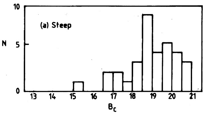
An example application of the test is shown in Fig. 7, which presents magnitude distributions for flat and steep (radio) spectrum QSOs. H₁ is that the flat-spectrum QSOs extend to significantly lower (brighter) magnitudes than do the steep-spectrum QSOs, a claim made earlier by several observers. The eye agrees with H₁, and so does the result from the U test, in which we found U = 719, z = 2.69, rejecting H₀ in favour of H₁ at the 0.004 level of significance.

Fig. 7. An application of the Mann-Whitney-Wilcoxon U test. The frequency distributions are magnitude histograms for a complete sample of QSOs from the Parkes 2.7-GHz survey (Masson & Wall 1977), (a) steep-spectrum objects, (b) flat-spectrum objects. H1 is that the flat-spectrum QSOs have stochastically smaller (brighter) magnitudes than the steep-spectrum QSOs. U = 719, z = 2.69; H0 is rejected at the 0.004 level of significance.

Critical values of D are given in Tables A VII and A VIII. Table A VII gives the values for small samples, one-tailed test, while Table A VIII is for the two-tailed test. For large samples, two-tailed test, use Table A IX. For large samples, one-tailed test, compute

which has a sampling distribution approximated by chi-square with two degrees of freedom. Then consult Table A III to see if the observed D results in a value of ² large enough to reject H₀ in favour of H₁ at the desired level of significance.

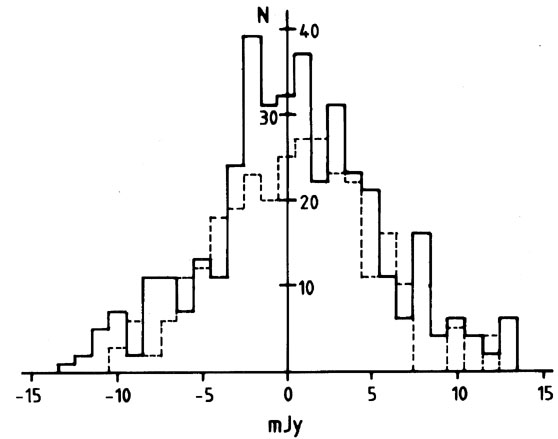
An example is shown in Fig. 8. The frequency distributions show the strengths of radio emission detected at particular positions in the sky. There was good (a priori!) reason to suspect that the positions observed in the larger sample should result in greater detected radio flux than the random positions of the smaller sample. The eye (a posteriori!) suggests that this might not actually be so. H₁ is that the distributions differ in the sense that observations of the larger sample stochastically exceed those of the smaller: H₀ = no difference. The Kolmogorov-Smirnov test yielded D = 0.068 for m = 290, n = 385. Hence ² = 3.06 for 2 degrees of freedom; the associated probability is 0.25, a very boring number, and quite inadequate to allow rejection of H₀ in favour of H₁.

Fig. 8. An application of the Kolmogorov-Smirnov two-sample test. Flux density measurements giving rise to the smaller sample were at random positions; those of the larger sample were not. The hypothesis that the distributions are the same (H0, there is no flux-density excess at the preferred positions) cannot be rejected in favour of H1 (the deflections of the larger sample are stochastically larger; there is excess flux density at the preferred positions). Dmax = 0.068 (at + 7 mJy) for m = 290, n = 385 and in the predicted sense. This yields 2 = 3.06 for 2 degrees of freedom, a probability of 25 per cent, no man's land.