Annu. Rev. Astron. Astrophys. 1994. 32: 371-418 Copyright © 1994 by Annual Reviews. All rights reserved

5. PREDICTED MOTIONS FROM THE GALAXY Z-DISTRIBUTION

All-sky complete redshift surveys provide extremely valuable data complementary to the peculiar velocity data, and the efficient techniques for measuring redshifts make them deeper, denser, and more uniform. Under the assumption of GI and an assumed biasing relation between galaxies and mass, a redshift survey enables an independent reconstruction of the density and velocity fields. The comparison of the smoothed fields recovered from redshifts and from velocities is a very important tool for testing the basic hypotheses and for determining the cosmological parameters.

The solution to the linearized GI equation · v = -f for an irrotational field is

v(x) = f / 4 _{all space} d³ x' (x') [(x' - x) / |x' - x|³]. (19)

The velocity is proportional to the gravitational acceleration, which ideally requires full knowledge of the distribution of mass in space. In practice (Yahil et al. 1991) one is provided with a flux-limited, discrete redshift survey, obeying some radial selection function (r). The galaxy density is estimated by 1 + _g(x) = n^-1 (r_i)^{-1 3}_dirac(x - x_i), where n V^-1 (r_i)^-1 is the mean galaxy density, and the inverse weighting by restores the equal-volume weighting. Equation (19) is then replaced by

v(x) = / 4 _{r < Rmax} d³ x' _g(x') S(|x' - x|) [(x' - x) / |x' - x|³]. (20)

Under the assumption of linear biasing, _g = b , the cosmological dependence enters through f() / b. The integration is limited to r < R_max where the signal dominates over shot-noise. S(x) is a small-scale smoothing window ( 500 km s^-1) essential for reducing the effects of non-linear gravity, shot-noise, distance uncertainty, and triple-value zones. The distances are estimated from the redshifts in the LG frame by

r_i = z_i - x_ihat · [v(x_i) - v(0)]. (21)

Equations (20-21) can be solved iteratively: make a first guess for the x_i, compute the v_i by Equation (20), correct the x_i by Equation (21), and so on until convergence. The convergence can be improved by increasing gradually during the iterations. Relevant issues follow.

SELECTION FUNCTION. An accurate knowledge of the probability that a galaxy at a given distance be included in the sample is essential, especially at large distances where ^-1 can introduce large errors. For a given flux limit, can be evaluated together with the luminosity function using a maximum-likelihood technique independent of density inhomogeneities.

ZONE OF AVOIDANCE. Regions in the sky not covered by the survey have to be filled with mock galaxies by some method of extrapolation from nearby regions. One way is to distribute these galaxies Poissonianly with the mean density of an adjacent volume, or to actually clone the adjacent region (Hudson 1993a). A more sophisticated extrapolation uses spherical harmonics and the Wiener filter method (e.g. Lahav et al. 1994).

TRIPLE-VALUED ZONES. Galaxies in three different positions along a line of sight through a contracting region may have the same redshift. Given a redshift in a collapsing region where the problem is not resolved by the smoothing used, one can either take some average of the three solutions, or make an intelligent choice between them, e.g. by using the velocity field derived from observed velocities.

ESTIMATING SHOT-NOISE. This major source of error due to the finite number of galaxies can be crudely estimated using bootstrap simulations, where each galaxy is replaced with k galaxies, k being a Poisson deviate of <k> = 1. For each realization one calculates and n, corrects for the ZOA, and solves for the linear velocity field. The mean and variance of the resulting density field are measures of the systematic and random errors. The bootstrap simulations demonstrate that the uncertainty in _g from the 1.2 Jy IRAS sample is typically less than 50% of the uncertainty in the density derived by POTENT from observed Mark III velocities.

NONLINEAR BIASING. Galaxies need not be faithful tracers of the mass (e.g. Dekel & Rees 1987), but there is growing evidence that they are strongly correlated (Section 6.2). This correlation can be crudely assumed to be a deterministic relation between the local smoothed density fields, e.g. linear biasing _g = b, which is one realization of the linear statistical relation between the variances of the fields predicted for linear density peaks in a Gaussian field (Kaiser 1984; Bardeen et al. 1986). However, a more sophisticated analysis may require a more realistic biasing relation, e.g. an exception from linear biasing which must be made for negative _g and b < 1 to prevent from falling unphysically below -1. The non-linear generalization 1 + _g = (1 + )^b is useful (e.g. Dekel et al. 1993) and it fits quite well The biasing seen in simulations of galaxy formation in a CDM scenario involving cooling and gas dynamics (Cen & Ostriker 1993), except that a small correction is needed to force the means of and _g to vanish simultaneously as required by definition.

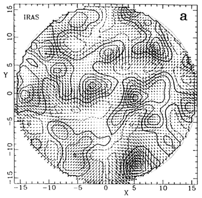
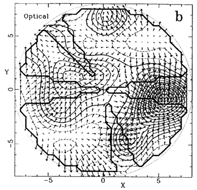
Figure 4. The fluctuation fields of galaxies in the Supergalactic plane as deduced from redshift surveys with 10 h-1Mpc smoothing. Distances and velocities are in km s-1. (a) Reconstructed by A. Yahil and M. Strauss using a power-preserving filter from the IRAS 1.2 Jy data in a sphere of radius 160 h-1Mpc. (b) Reconstructed by Hudson (1993a, 1994) from optical data within 80 h-1Mpc, extrapolated into the unsampled areas ouside the heavy contour.

QUASILINEAR CORRECTION. Even after 12 h^-1Mpc smoothing, _g is of order unity in places, necessitating a quasi-linear treatment. Local approximations from v to were discussed in Section 2, but the non-local nature of the inverse problem makes it less straightforward. A possible solution is to find an inverse relation of the sort · v = F(, _g), including non-linear biasing and non-linear gravity. This is a Poisson-like equation in which - _g(x) is replaced by F(x), and since the smoothed velocity field is irrotational for quasi-linear perturbations as well, it can be integrated analogously to Equation (20). With smoothing of 10 h^-1Mpc and = 1, the approximation based on _c has an rms error < 50 km s^-1 (Mancinelli et al. 1994). Note that for very small b the associated with the observed _g could be non-linear to the extent that the quasi-linear approximations break down. When is given, the Poisson equation can be integrated more efficiently by using grid-based FFT techniques than by straightforward summation. The r-space (x) deduced from the z-space galaxy distribution is not too sensitive to non-linear effects or the value of , so it is a reasonable shortcut to correct for non-linear effects only in the transformation from to v using FFT.

The IRAS Point Source Catalog served as the source for two very valuable redshift surveys, which have been carried out and analyzed in parallel. One contains the 5313 galaxies brighter than 1.2 Jy at 60µm with sky coverage (almost) complete for |b| > 5° covering 88% of the sky (Strauss et al. 1990, 1992a, to 1.9 Jy; extended by Fisher 1992). The other is a 1-in-6 sparsely-sampled survey of 2300 galaxies down to the IRAS flux limit of 0.6 Jy (Rowan-Robinson et al. 1990, QDOT), which is now being extended to a fully-sampled survey (Saunders et al. in preparation). As for optical galaxies, Hudson (1993a) developed a clever way to reconstruct a statistically uniform density field out to ~ 80 h^-1Mpc by combining the UGC/ESO diameter-limited angular catalogs and the ZCAT incomplete redshift survey. Figure 4 shows maps of the galaxy density fields and the associated predicted velocity fields, with the main features corresponding to those recovered from observed velocities (Figure 3), e.g. the GA, PP and Coma superclusters and the voids in between (Section 6.2).