4. TESTING COSMOLOGICAL GAUSSIANITY

Largely motivated by the idea that they were generated by quantum fluctuations during a period of inflation, most fashionable models of structure formation involve the assumption that the initial fluctuations constitute a Gaussian random field. Mathematically, this assumption means that all finite- dimensional joint probability distributions of the density at different spatial locations can be expressed as multivariate normal distributions. This is much stronger than the assertion that the distribution of densities should be a normal distribution. It is quite possible for a field to have a Gaussian one-point probability distribution but be non-Gaussian in the sense used here. Testing this form of multivariate normality in an arbitrary number of dimensions is a decidedly non-trivial task, but is necessary given the importance of the assumption. If it can be shown that the large-scale structure of the Universe is inconsistent with Gaussian initial data this will have profound implications for fundamental physics. This issue does not therefore represent a mere exercise in statistics, but a vital step towards a physical understanding of the origin and evolution of the large-scale structure of the Universe.

As well as being physically motivated, the Gaussian assumption has great advantage that it is a mathematically complete prescription for all the statistical properties of the initial density field, once the fluctuation amplitude is specified as a function of scale through the power-spectrum P(k). In Fourier terms, a Gaussian random field consists of a stochastic superposition of plane waves. The amplitude of each mode, A_k, is drawn from a distribution specified by the power-spectrum and its phase, _k, is uniformly random and independent of the phases of all other modes. As the fluctuations evolve in time, the density distribution becomes non-Gaussian. But this departure from non-Gaussianity depends on gravity being able to move material from its primordial position. On scales much larger than the typical scale of such motions, the distribution remains Gaussian. The distribution of matter today should therefore be highly non-Gaussian on small scales, gradually tending closer to Gaussian on progressively larger scales. Any non-Gaussianity detected at the present epoch could therefore either be primordial, or produced dynamically, or could could be imposed by variations in mass-to-light ratio (bias), or all of these. Galaxy clustering statistics therefore need to be devised that can separate these different signatures.

The distribution of temperature fluctuations in the cosmic microwave background (CMB), which was imprinted before significant gravitational evolution took place, should also retain the character of the initial statistics. Any non-Gaussianity detected here could either be primordial, produced by errors in foreground subtraction or other systematics. Again, tests capable of distinguishing between these possibilities are required.

Gaussian models have generally fared much better in comparison with data than others with non-Gaussian initial data, such as those based on topological defects, although predictions in the second category of models are harder to come by because of the much greater calculational difficulties involved. It is fair to say, however, that as far as existing data are concerned the large-scale distribution of mass certainly seems to be consistent with Gaussian statistics. Initially, it also appeared that the COBE fluctuations in temperature of the CMB were also consistent with Gaussian primordial perturbations. On the other hand, the statistical descriptors necessary to carry out a powerful test against the Gaussian require much higher quality data than has so far been furnished by galaxy surveys. Moreover, the non-Gaussianity induced by gravitational evolution, redshift-space effects, and variations in mass-to-light ratio has complicated the interpretation of the data, although recent theoretical developments discussed below should ameliorate these problems.

In the following I discuss a method of quantifying phase information [Chiang & Coles 2000] and suggest how this information may be exploited to build novel statistical descriptors that can be used to mine the sky more effectively than with standard methods.

4.1. Fourier Description of Cosmological Density Fields

In most popular versions of the ``gravitational instability'' model for the origin of cosmic structure, particularly those involving cosmic inflation [Guth & Pi 1982], the initial fluctuations that seeded the structure formation process form a Gaussian random field [Bardeen et al. 1986]. Because the initial perturbations evolve linearly, it is useful to expand (x) as a Fourier superposition of plane waves:

(25)

The Fourier transform (k) is complex and therefore possesses both amplitude |(k)| and phase _k where

(26)

Gaussian random fields possess Fourier modes whose real and imaginary parts are independently distributed. In other words, they have phase angles _k that are independently distributed and uniformly random on the interval [0, 2]. When fluctuations are small, i.e. during the linear regime, the Fourier modes evolve independently and their phases remain random. In the later stages of evolution, however, wave modes begin to couple together [Peebles 1980]. In this regime the phases become non-random and the density field becomes highly non-Gaussian. Phase coupling is therefore a key consequence of nonlinear gravitational processes if the initial conditions are Gaussian and a potentially powerful signature to exploit in statistical tests of this class of models.

A graphic demonstration of the importance of phases in patterns generally is given in Fig 2. Since the amplitude of each Fourier mode is unchanged in the phase reshuffling operation, these two pictures have exactly the same power-spectrum, P(k) |(k)|². In fact, they have more than that: they have exactly the same amplitudes for all k. They also have totally different morphology. Further demonstrations of the importance of Fourier phases in defining clustering morphology are given by Chiang (2001). The evident shortcomings of P(k) can be partly ameliorated by defining higher-order quantities such as the bispectrum [Peebles 1980, Matarrese et al. 1997, Scoccimarro et al. 1999, Verde et al. 2000] or correlations of (k)² [Stirling & Peacock 1996].

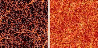
Figure 2. Numerical simulation of galaxy clustering (left) together with a version generated randomly reshuffling the phases between Fourier modes of the original picture (right).

4.2. The Bispectrum and Phase Coupling

The bispectrum and higher-order polyspectra vanish for Gaussian fields, but in a non-Gaussian field they may be non-zero. The usefulness of these and related quantities therefore lies in the fact that they encode some information about non-linearity and non-Gaussianity. To understand the relationship between the bispectrum and Fourier phases, it is very helpful to consider the following toy examples. Imagine a simple density field defined in one spatial dimension that consists of the superposition of two cosine components:

(27)

The generalisation to several spatial dimensions is trivial. The phases ₁ and ₂ are random and A₁ and A₂ are constants. We can simplify the following by introducing a new notation

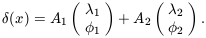
(28)

Clearly this example displays no phase correlations. Now consider a new field obtained from the example (27) through the non-linear transformation

(29)

where is a constant parameter. Equation (29) may be thought of as a very phenomenological representation of a perturbation series, with controlling the level of non-linearity. Using the same notation as equation (28), the new field (x) can be written

(30)

where the B_i are constants obtained from the A_i. Notice in equation (30) that the phases follow the same kind of harmonic relationship as the wavenumbers. This form of phase association is termed quadratic phase coupling. It is this form of phase relationship that appears in the bispectrum. To see this, consider another two toy examples. First, model A,

(31)

in which ₃ = ₁ + ₂ but in which ₁, ₂ and ₃ are random; and

(32)

Model A exhibits no phase association; model B displays quadratic phase coupling. It is straightforward to show that < _A > = < _B > = 0. The autocovariances are equal:

(33)

as are the power spectra, demonstrating that second-order statistics are blind to phase association. The (reduced) three-point autocovariance function is

(34)

For model A we get

(35)

whereas for model B it is

(36)

The bispectrum, B(k₁, k₂), is defined as the two-dimensional Fourier transform of , so B_A(k₁, k₂) = 0 trivially, whereas B_B(k₁, k₂) consists of a single spike located somewhere in the region of (k₁, k₂) space defined by k₂ 0, k₁ k₂ and k₁ + k₂ . If _{1 2} then the spike appears at k₁ = ₁, k₂ = ₂). Thus the bispectrum measures the phase coupling induced by quadratic nonlinearities. To reinstate the phase information order-by-order requires an infinite hierarchy of polyspectra.

An alternative way of looking at this issue is to note that the information needed to fully specify a non-Gaussian field to arbitrary order (or, in a wider context, the information needed to define an image resides in the complete set of Fourier phases [Oppenheim & Lim 1981]. Unfortunately, relatively little is known about the behaviour of Fourier phases in the nonlinear regime of gravitational clustering [Ryden & Gramman 1991, Scherrer et al. 1991, Soda & Suto 1992, Jain & Bertschinger 1996, Jain & Bertschinger 1998, Coles & Chiang 2000], but it is of great importance to understand phase correlations in order to design efficient statistical tools for the analysis of clustering data.

4.3. Visualizing and Quantifying Phase Information

A vital first step on the road to a useful quantitative description of phase information is to represent it visually [Coles & Chiang 2000]. In colour image display devices, each pixel represents the intensity and colour at that position in the image [Thornton 1998, Foley & Van Dam 1982]. The quantitative specification of colour involves three coordinates describing the location of that pixel in an abstract colour space, designed to reflect as accurately as possible the eye's response to light of different wavelengths. In many devices this colour space is defined in terms of the amount of Red, Green or Blue required to construct the appropriate tone; hence the RGB colour scheme. The scheme we are particularly interested in is based on three different parameters: Hue, Saturation and Brightness. Hue is the term used to distinguish between different basic colours (blue, yellow, red and so on). Saturation refers to the purity of the colour, defined by how much white is mixed with it. A saturated red hue would be a very bright red, whereas a less saturated red would be pink. Brightness indicates the overall intensity of the pixel on a grey scale. The HSB colour model is particularly useful because of the properties of the `hue' parameter, which is defined as a circular variable. If the Fourier transform of a density map has real part R and imaginary part I then the phase for each wavenumber, given by = arctan(I / R), can be represented as a hue for that pixel using the colour circle [Coles & Chiang 2000].

The pattern of phase information revealed by this method related to the gravitational dynamics of its origin. For example in our analysis of phase coupling [Chiang & Coles 2000] we introduced a quantity D_k, defined by

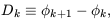
(37)

which measures the difference in phase of modes with neighbouring wavenumbers in one dimension. We refer to D_k as the phase gradient. To apply this idea to a two-dimensional simulation we simply calculate gradients in the x and y directions independently. Since the difference between two circular random variables is itself a circular random variable, the distribution of D_k should initially be uniform. As the fluctuations evolve waves begin to collapse, spawning higher-frequency modes in phase with the original [Shandarin & Zel'dovich 1989]. These then interact with other waves to produce a non-uniform distribution of D_k. For examples, see

http://www.nottingham.ac.uk/~ppzpc/phases/index.html.

It is necessary to develop quantitative measures of phase information that can describe the structure displayed in the colour representations. In the beginning the phases _k are random and so are the D_k obtained from them. This corresponds to a state of minimal information, or in other words maximum entropy. As information flows into the phases the information content must increase and the entropy decrease. One way to quantify this is by defining an information entropy on the set of phase gradients. One constructs a frequency distribution, f (D) of the values of D_k obtained from the whole map. The entropy is then defined as

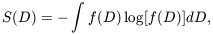
(38)

where the integral is taken over all values of D, i.e. from 0 to 2. The use of D, rather than itself, to define entropy is one way of accounting for the lack of translation invariance of , a problem that was missed in previous attempts to quantify phase entropy [Polygiannikis & Moussas 1995]. A uniform distribution of D is a state of maximum entropy (minimum information), corresponding to Gaussian initial conditions (random phases). This maximal value of S_max = log(2) is a characteristic of Gaussian fields. As the system evolves it moves into to states of greater information content (i.e. lower entropy). The scaling of S with clustering growth displays interesting properties [Chiang & Coles 2000], establishing an important link between the spatial pattern and the physics driving clustering growth.