


Regular motion is defined as motion that respects at least N
isolating integrals, where N is the number of degrees of freedom
(DOF), i.e. the dimensionality of configuration space.
Regular motion can always be reduced to translation on a torus;
that is, a canonical transformation
(x, v) -> (J,
 ) can be found such that
| (6) |
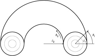
The constants Ji, called the actions, define the radii of
the various cross-sections of the torus while the angles
i define the
position on the torus (Figure 1).
The dimensionality of a torus is therefore equal to that
of an orbit in configuration space.
Each point on an orbit maps to 2N points on its torus;
for N = 2, these four points correspond to the four velocity
vectors (± vx, ± vy)
through a given configuration space point.
The  i are called
fundamental frequencies; in the generic case, they are incommensurable,
i.e. their ratios can not be expressed as ratios of integers.
Orbits defined by incommensurable frequencies map onto the entire
surface of the torus, filling it densely after a sufficiently long time.
For certain orbits, a resonance between the fundamental frequencies
occurs, i.e.
n . = 0 with
n = (l, m) a nonzero integer vector.
In two degrees of freedom such a resonance implies
1 /
2 =
|m/l| and the orbit is periodic, closing on itself after
|m| revolutions in
1 and | l|
revolutions in 2.
When N > 2, each independent resonance condition reduces the
dimensionality of the orbit by one, and N - 1 such conditions are
required for closure. With the exception of special Hamiltonians like
the spherical harmonic oscillator, resonant tori comprise a set of measure
zero, although they are dense in the phase space.
i are called
fundamental frequencies; in the generic case, they are incommensurable,
i.e. their ratios can not be expressed as ratios of integers.
Orbits defined by incommensurable frequencies map onto the entire
surface of the torus, filling it densely after a sufficiently long time.
For certain orbits, a resonance between the fundamental frequencies
occurs, i.e.
n . = 0 with
n = (l, m) a nonzero integer vector.
In two degrees of freedom such a resonance implies
1 /
2 =
|m/l| and the orbit is periodic, closing on itself after
|m| revolutions in
1 and | l|
revolutions in 2.
When N > 2, each independent resonance condition reduces the
dimensionality of the orbit by one, and N - 1 such conditions are
required for closure. With the exception of special Hamiltonians like
the spherical harmonic oscillator, resonant tori comprise a set of measure
zero, although they are dense in the phase space.
|
Figure 1. Invariant torus defining the
motion of a regular orbit in a two-dimensional potential.
The torus is determined by the values of the actions
J1 and
J2; the position of the trajectory on the torus is
defined by
the angles |
In potentials that support N global integrals, like that of the Perfect Ellipsoid, all trajectories lie on tori and the Hamiltonian can be written

| (7) |
with
| (8) |
The tori of an integrable system are nested in a completely regular way throughout phase space. According to the KAM theorem, these tori will survive under small perturbations of H if their frequencies are sufficiently incommensurable ([Lichtenberg & Lieberman 1992]). Resonant tori may be strongly deformed even under small perturbations, however, leading to a complicated phase-space structure of interleaved regular and chaotic regions. Where tori persist, the motion can be characterized in terms of N local integrals. Where tori are destroyed, the motion is chaotic and the orbits move in a space of higher dimensionality than N.
While (local) action-angle variables are guaranteed to exist if the motion
is regular, there is no general, analytic technique for calculating the
(J, ) from the
(x, v).
This is unfortunate since the representation of an orbit in terms
of its action-angle variables is maximally compact, reducing the
2N - 1 variables on the energy surface to just N angles.
In addition, time-averaged quantities become trivial to compute
since the probability
of finding a star on the torus is uniform in the angle variables.
For instance, the configuration space density is
| (9) |
which can be trivially evaluated given
x().
Finally, the actions are conserved under slow deformations of the
potential, a useful property if one wishes to compute the
evolution of a galaxy that is subject to some gradual perturbing force.
Fortunately, a number of algorithms have been developed in recent years for numerically extracting the relations between the Cartesian and action-angle variables. Most of this work has been directed toward 2 DOF systems, making it applicable to axisymmetric potentials or to motion in a principal plane of a nonrotating triaxial galaxy. Generalizations to three degrees of freedom are straightforward in principle, although in practice some of the algorithms described here become inefficient when N > 2.
In canonical perturbation theory, one begins by writing the Hamiltonian as the sum of two terms,
| (10) |
where H0 is integrable and
 is a
(hopefully small) perturbation parameter.
One then seeks a canonical transformation to new action-angle
variables such that the Hamiltonian is independent of
.
The transformation is found by expanding the generating function in
powers of and solving
the Hamilton-Jacobi equation successively to each order.
The KAM theorem states that such a transformation will
sometimes exist, at least when
is sufficiently small
and when the unperturbed
i are
sufficiently far from commensurability.
In a system with one degree of freedom, this approach is equivalent to
Lindstedt's (1882)
method in which both the
amplitude and frequency of the oscillation are expanded as
power series in ; the
result is a uniformly convergent series solution for the motion.
Davoust (1983a,
b,
c) and
Scuflaire (1995)
presented applications
of Lindstedt's method to periodic motion in simple galactic potentials.
is a
(hopefully small) perturbation parameter.
One then seeks a canonical transformation to new action-angle
variables such that the Hamiltonian is independent of
.
The transformation is found by expanding the generating function in
powers of and solving
the Hamilton-Jacobi equation successively to each order.
The KAM theorem states that such a transformation will
sometimes exist, at least when
is sufficiently small
and when the unperturbed
i are
sufficiently far from commensurability.
In a system with one degree of freedom, this approach is equivalent to
Lindstedt's (1882)
method in which both the
amplitude and frequency of the oscillation are expanded as
power series in ; the
result is a uniformly convergent series solution for the motion.
Davoust (1983a,
b,
c) and
Scuflaire (1995)
presented applications
of Lindstedt's method to periodic motion in simple galactic potentials.
In systems with two or more degrees of freedom,
the transformation to action-angle variables is not usually
expressible as a power series in
.
The reason is the "problem of small denominators": a Fourier
expansion of H1 in terms of the
i will generally
contain terms with n .
 0 which
cause the perturbation series to blow up.
This phenomenon is indicative of a real change in the structure
of phase space near resonances: if the perturbation parameter
is small,
H0 +
H1 can be topologically
different from H0 only if H1 is large.
However, a number of techniques have been developed to formally
suppress the divergence.
One approach, called secular perturbation theory, is
useful near resonances in the unperturbed Hamiltonian,
l 1 +
m2 = 0.
One first transforms to a frame that rotates with the resonant
frequency; in this frame, the new angle variable measures
the slow deviation from resonance. The Hamiltonian is then averaged over
the other, fast angle variable.
To lowest order in , the
new action is lJ2 + mJ1 and
the motion in the slow variable can be found by quadrature.
Solutions obtained in this way are asymptotic approximations to the
exact ones, i.e. they differ from them by at most
O()
for times of order
-1.
Whether they are good descriptions of the actual motion depends
on the strength of the perturbation and the timescale of interest.
0 which
cause the perturbation series to blow up.
This phenomenon is indicative of a real change in the structure
of phase space near resonances: if the perturbation parameter
is small,
H0 +
H1 can be topologically
different from H0 only if H1 is large.
However, a number of techniques have been developed to formally
suppress the divergence.
One approach, called secular perturbation theory, is
useful near resonances in the unperturbed Hamiltonian,
l 1 +
m2 = 0.
One first transforms to a frame that rotates with the resonant
frequency; in this frame, the new angle variable measures
the slow deviation from resonance. The Hamiltonian is then averaged over
the other, fast angle variable.
To lowest order in , the
new action is lJ2 + mJ1 and
the motion in the slow variable can be found by quadrature.
Solutions obtained in this way are asymptotic approximations to the
exact ones, i.e. they differ from them by at most
O()
for times of order
-1.
Whether they are good descriptions of the actual motion depends
on the strength of the perturbation and the timescale of interest.
Verhulst (1979)
applied the averaging technique to
motion in the meridional plane of an axisymmetric galaxy.
He expanded the potential in a quartic polynomial about
the circular orbit in the plane, thus restricting his results to
epicyclic motion but at the same time guaranteeing a finite
Fourier expansion for H1.
He related the fundamental frequencies by setting
z2 =
(r/s)2
x2 +
 () and found solutions to
first order in
for various
choices of the integers (r, s).
For r = s = 1 he recovered
Contopoulos's (1960)
famous "third integral," as well as
Saaf's (1968)
formal integral for a quartic potential.
De Zeeuw &
Merritt (1983)
and de Zeeuw (1985a)
applied Verhulst's formalism to motion near the center of a triaxial
galaxy with an analytic core. Here the unperturbed
i are the
frequencies of harmonic oscillation near the center.
De Zeeuw & Merritt showed
that the choice r = s = 1 produced a reasonable
representation of the orbital structure in the plane of rotation,
including the important 1 : 1 closed loop orbits that generate the
three-dimensional tubes.
Robe (1985,
1986,
1987)
used an exact technique to recover the periodic orbits in the case of 1
: 1 : 1 resonance and investigated their stability.
() and found solutions to
first order in
for various
choices of the integers (r, s).
For r = s = 1 he recovered
Contopoulos's (1960)
famous "third integral," as well as
Saaf's (1968)
formal integral for a quartic potential.
De Zeeuw &
Merritt (1983)
and de Zeeuw (1985a)
applied Verhulst's formalism to motion near the center of a triaxial
galaxy with an analytic core. Here the unperturbed
i are the
frequencies of harmonic oscillation near the center.
De Zeeuw & Merritt showed
that the choice r = s = 1 produced a reasonable
representation of the orbital structure in the plane of rotation,
including the important 1 : 1 closed loop orbits that generate the
three-dimensional tubes.
Robe (1985,
1986,
1987)
used an exact technique to recover the periodic orbits in the case of 1
: 1 : 1 resonance and investigated their stability.
Gerhard & Saha
(1991)
compared the usefulness of three
perturbative techniques for reproducing the meridional-plane motion in
axisymmetric models. They considered: (1)
Verhulst's (1979)
averaging technique; (2) a resonant method based on Lie transforms; and
(3) a "superconvergent" method. The latter was proposed originally by
Kolmogorov (1954)
and developed by
Arnold (1963) and
Moser (1967)
in their proof of the KAM theorem.
The KAM method can only generate orbit families that are
present in H0.
Gerhard & Saha took for their unpertured potential the spherical
isochrone and set
 1 =
g(r) P20(cos).
They were able to reproduce the main features of the
motion using the resonant Lie transform method, including the
box orbits that are not present when
1 = 0.
The KAM method could only generate loop orbits but did so
with great accuracy when taken to high order.
Dehnen & Gerhard
(1993)
used the approximate integrals generated
by the resonant Lie-transform method to construct three-integral
models of axisymmetric galaxies, as described in
Section 3.3.
1 =
g(r) P20(cos).
They were able to reproduce the main features of the
motion using the resonant Lie transform method, including the
box orbits that are not present when
1 = 0.
The KAM method could only generate loop orbits but did so
with great accuracy when taken to high order.
Dehnen & Gerhard
(1993)
used the approximate integrals generated
by the resonant Lie-transform method to construct three-integral
models of axisymmetric galaxies, as described in
Section 3.3.
2.1.2. Nonperturbative Methods
The failure of perturbation expansions to converge reflects the change in phase space topology that occurs near resonances in the unperturbed Hamiltonian. As an alternative to perturbation theory, one can assume that a given orbit is confined to a torus and solve directly for the action-angle variables in terms of x and v. If the orbit is indeed regular, such a solution is guaranteed to exist and corresponds to a perturbation expansion carried out to infinite order (assuming the latter is convergent). For a chaotic orbit, the motion is not confined to a torus but one might still hope to derive an approximate torus that represents the average behavior of a weakly chaotic trajectory over some limited interval of time.
Ratcliff, Chang & Schwarzschild (1984) pioneered this approach in the context of galactic dynamics. They noted that the equations of motion of a 2D orbit,
| (11) |
can be written in the form
| (12) |
where
1 =
1t and
2 =
2t, the
coordinates on the torus. If one specifies
1 and
2 and treats
ð / ðx and
ð / ðy as
functions of the i, equations (12) can be
viewed as nonlinear equations for
x(1,
2) and
y(1,
2).
No very general method of solution exists for such equations;
iteration is required and success depends on the stability of the
iterative scheme. Ratcliff et al. chose to express the coordinates as
Fourier series in the angle variables,
| (13) |
Substituting (13) into (12) gives
| (14) |
where the right hand side is again understood to be a function of the angles. Ratcliff et al. truncated the Fourier series after a finite number of terms and required equations (14) to be satisfied on a grid of points around the torus. They then solved for the Xn by iterating from some initial guess. Convergence was found to be possible if the initial guess was close to the exact solution. Guerra & Ratcliff (1990) applied a similar algorithm to orbits in the plane of rotation of a nonaxisymmetric potential.
Another iterative approach to torus reconstruction was first
developed in the context of semiclassical quantum theory by
Chapman, Garrett &
Miller (1976).
Binney and collaborators
([McGill & Binney
1990];
[Binney & Kumar
1993];
[Kaasalainen &
Binney 1994a],
1994b;
[Kaasalainen 1994],
1995a,
b)
further developed the technique and applied it to galactic potentials.
One starts by dividing the Hamiltonian H into separable and
non-separable parts H0 and H1, as in
equation (10); however
H1 is
no longer required to be small.
One then seeks a generating function S that maps the known tori
of H0 into tori of H.
For a generating function of the F2-type
(Goldstein 1980),
one has
| (15) |
where (J, ) and
(J', ')
are the action-angle variables of H0 and H
respectively.
The generator S is determined, for a specified J',
by substituting the first of equations (15) into the Hamiltonian
H(J, ) and
requiring the result to be independent of
. One then arrives at
H(J').
Chapman et al. showed that a sufficiently general form for S is
| (16) |
where the first term is the identity transformation, and they evaluated a number of iterative schemes for finding the Sn. One such scheme was found to recover the results of first-order perturbation theory after a single iteration.
The generating function approach is useful for assigning energies
to actions, H(J'), but most of the other quantities of
interest to galactic dynamicists require additional effort.
For instance, equation (15) gives
'()
as a derivative of S, but since S must be computed separately
for every J' its derivative is likely to be ill-conditioned.
Binney & Kumar
(1993) and
Kaasalainen &
Binney (1994a)
discussed two schemes for finding
'(); the first
required the solution of a formally infinite set of equations, while the
latter required multiple integrations of the equations of motion
for each torus.
Another feature of the generating function approach is its lack of robustness. Kaasalainen & Binney (1994a) noted that the success of the method depends somewhat on the choice of H0. For box orbits, which are most naturally described as coupled rectilinear oscillators, they found that a harmonic-oscillator H0 gave poor results unless an additional point transformation was used to deform the rectangular orbits of H0 into narrow-waisted boxes like those in typical galactic potentials. Kaasalainen (1995a) considered orbits belonging to higher-order resonant families and found that it was generally necessary to define a new coordinate transformation for each family.
Warnock (1991)
presented a modification of the Chapman et al.
algorithm in which the generating funtion S was
derived by numerically integrating an orbit from appropriate
initial conditions, transforming the coordinates to
(J, ) of
H0 and interpolating J on a regular grid in
.
The values of the Sn then follow from the
first equation of (15) after a discrete Fourier transform.
Kaasalainen &
Binney (1994b)
found that Warnock's scheme could be
used to substantially refine the solutions found via their iterative
scheme.
Having computed the energy on a grid of J' values, one can interpolate to obtain the full Hamiltonian H(J'1, J'2). If the system is not in fact completely integrable, this H may be rigorously interpreted as smooth approximation to the true H ([Warnock & Ruth 1991], 1992) and can be taken as the starting point for secular perturbation theory. Kaasalainen (1994, 1995b) developed this idea and showed how to recover accurate surfaces of section in the neighborhood of low-order resonances in the planar logarithmic potential.
Percival (1977) described a variational principle for constructing tori. His technique has apparently not been implemented in the context of galactic dynamics.
2.2. Trajectory-Following Approaches
A robust and powerful alternative to the generating function approach is to construct tori by Fourier decomposition of the trajectories. Trajectory-following algorithms are based on the fact that integrable motion is quasiperiodic; in other words, in any canonical coordinates (p, q), the motion can be expressed as
| (17) |
where the i are
the N fundamental frequencies on the torus.
It follows from equations (17) that the Fourier transform of
x(t) or
v(t) will consist of a set of spikes at discrete frequencies
k that are linear
combinations of the fundamental frequencies.
An analysis of the frequency spectrum yields both the fundamental
frequencies and the integer vectors n associated with each spike.
The relation between the Cartesian coordinates and the angles
follows immediately from equation (17).
For instance, the x coordinate in a 2 DOF system becomes
| (18) |
and similarly for y(t). The actions can be computed from Percival's (1974) formulae,
| (19) |
thus yielding the complete map (x,v) -> (J,
).
Binney & Spergel
(1982)
pioneered the trajectory-following
approach in galactic dynamics, using a least-squares algorithm to
compute the Xk.
They were able to recover the fundamental frequencies in a 2 DOF
potential with a modest accuracy of ~ 0.1% after ~ 25 orbital periods.
Binney & Spergel
(1984)
used Percival's formula to construct the
action map for orbits in a principal plane of the logarithmic potential.
A major advance in trajectory-following algorithms was made by Laskar (1988, 1990), who developed a set of tools, the "numerical analysis of fundamental frequencies" (NAFF), for extracting the frequency spectra of quasiperiodic systems with very high precision. The NAFF algorithm consists of the following steps:
k will be defined
to an accuracy of ~ 1/MT.
| (20) |
where  (t) = 1 +
cos(2
(t) = 1 +
cos(2 t/T) is the
Hanning window function.
The integral can be approximated by interpolating the
discretely-sampled f (t).
The Hanning filter broadens the peak but greatly
reduces the sidelobes, allowing a very precise determination of
k.
t/T) is the
Hanning window function.
The integral can be approximated by interpolating the
discretely-sampled f (t).
The Hanning filter broadens the peak but greatly
reduces the sidelobes, allowing a very precise determination of
k.
kt onto
f (t), and subtract this component from the time series.
jt will not be mutually
orthogonal, a Gram-Schmidt procedure is used to construct orthonormal basis
functions before carrying out the projection in step 4.
k.
Laskar's algorithm recovers the fundamental frequencies with an error that falls off as T-4 ([Laskar 1996]), compared with ~ T-1 in algorithms like Binney & Spergel's (1982). Even for modest integration times of ~ 102 orbital periods, the NAFF algorithm is able to recover fundamental frequencies with an accuracy of ~ 10-8 or better. Such extraordinary precision allows the extraction of a large number of components from the frequency spectrum, hence a very precise representation of the torus.
Papaphilippou & Laskar (1996) applied the NAFF algorithm to 2DOF motion in a principal plane of the logarithmic potential. They experimented with different choices for the quantity f whose time series is used to compute the frequency spectrum. Ideally, one would choose f to be an angle variable, in terms of which the frequency spectrum reduces to a single peak, but the angles are not known a priori and the best one can do is to use the angle variables corresponding to some well-chosen Hamiltonian. However Papaphilippou & Laskar found that the convergence of the quasiperiodic expansion was only weakly affected by the choice of f; for most orbits, Cartesian coordinates (or polar coordinates in the case of loop orbits) were found to work almost as well as other choices. This result implies that trajectory-following methods are more easily automated than generating function methods which require a considerable degree of cleverness in the choice of coordinates.
Papaphilippou &
Laskar (1996)
focussed on the fundamental frequencies rather than the actions
for their characterization of the tori,
in part because the frequencies can be obtained with more precision
than the actions,
but also because KAM theory predicts that the structure of phase
space is determined in large part by resonances between the
i.
They defined the "frequency map," the curve of
2 /
1
values determined by a set of orbits of a given energy;
this curve is discontinuous whenever the initial conditions pass
over a resonance associated with chaotic motion.
The important resonances, and the sizes of their associated
chaotic regions, are immediately apparent from the frequency map.
Papaphilippou & Laskar showed that most of the chaos in the
logarithmic potential was
associated with the unstable short-axis orbit, a 1 : 1 resonance,
but they were also able to identify significant chaotic zones
associated with higher-order resonances like the 1 : 2 banana orbit.
One shortcoming of trajectory-following algorithms is that they
must integrate long enough for the orbit to adequately sample its
torus. When the torus is nearly resonant,
n .
0, the orbit is restricted
for long periods of time to a subset of the torus and the required
integration interval increases by a factor
~ 1/n . .
Another problem is the need to sample the time series with very high
frequency in order to minimize the effects of aliasing.