


Motion in an axisymmetric potential is qualitatively simpler than in a fully triaxial one due to conservation of angular momentum about the symmetry axis. Defining the effective potential
| (21) |
where
(R, z,  ) are
cylindrical coordinates and
Lz = R2
) are
cylindrical coordinates and
Lz = R2
 = constant,
the equations of motion are
= constant,
the equations of motion are
| (22) |
and
= Lz /
R2.
These equations describe the two-dimensional motion of a star in
the (R, z), or meridional, plane which rotates
non-uniformly about the symmetry axis.
Motion in axisymmetric potentials is therefore a 2 DOF problem.
Every trajectory in the meridional plane is constrained
by energy conservation to lie within the zero-velocity curve, the
set of points satisfying
E =  eff(R,
z). While the equations of motion (22) can not be solved in closed
form for arbitrary (R,
z), numerical integrations demonstrate that
most orbits do not densely fill the zero-velocity curve but instead
remain confined to narrower, typically wedge-shaped regions
([Ollongren 1962]);
in three dimensions, the orbits are tubes around
the short axis. (1)
The restriction of the motion to a subset of the region defined
by conservation of E and Lz is indicative of
the existence of an additional conserved quantity, or third integral
I3, for the majority of orbits.
Varying I3 at fixed E and Lz
is roughly equivalent to varying the height above and below
the equatorial plane of the orbit's
intersection with the zero velocity curve.
In an oblate potential, extreme values of I3
correspond either to orbits in the equatorial plane, or to "thin tubes,"
orbits which have zero radial action and which reduce to precessing
circles in the limit of a nearly spherical potential.
In prolate potentials, two families of thin tube orbits may exist:
"outer" thin tubes, similar to the thin tubes in oblate potentials,
and "inner" thin tubes, orbits similar to helices that wind
around the long axis
([Kuzmin 1973]).
eff(R,
z). While the equations of motion (22) can not be solved in closed
form for arbitrary (R,
z), numerical integrations demonstrate that
most orbits do not densely fill the zero-velocity curve but instead
remain confined to narrower, typically wedge-shaped regions
([Ollongren 1962]);
in three dimensions, the orbits are tubes around
the short axis. (1)
The restriction of the motion to a subset of the region defined
by conservation of E and Lz is indicative of
the existence of an additional conserved quantity, or third integral
I3, for the majority of orbits.
Varying I3 at fixed E and Lz
is roughly equivalent to varying the height above and below
the equatorial plane of the orbit's
intersection with the zero velocity curve.
In an oblate potential, extreme values of I3
correspond either to orbits in the equatorial plane, or to "thin tubes,"
orbits which have zero radial action and which reduce to precessing
circles in the limit of a nearly spherical potential.
In prolate potentials, two families of thin tube orbits may exist:
"outer" thin tubes, similar to the thin tubes in oblate potentials,
and "inner" thin tubes, orbits similar to helices that wind
around the long axis
([Kuzmin 1973]).
The area enclosed by the zero velocity curve tends to zero as
Lz approaches Lc(E), the
angular momentum of a circular orbit in the equatorial plane.
In this limit, the orbits may be viewed as perturbations of
the planar circular orbit, and an additional isolating integral
can generally be found
([Verhulst 1979]).
As Lz is reduced at fixed E, the amplitudes of
allowed motions in R and z increases and resonances
between the two degrees of freedom begin to appear.
Complete integrability is unlikely in the presence of resonances,
and in fact one can find often small regions of stochasticity at
sufficiently low Lz in axisymmetric potentials.
However the fraction of phase space associated with chaotic
motion typically remains small unless Lz is close to zero
([Richstone 1982];
[Lees &
Schwarzschild 1992];
[Evans 1994]).
The most important resonances at low Lz in oblate
potentials are
 z /
R = 1 : 1, which
produces the banana orbit in the meridional plane, and
z /
R = 3 : 4, the
fish orbit. The banana orbit bifurcates from the R-axial
(i.e. planar) orbit at high E and low Lz,
causing the latter to lose its stability;
the corresponding three-dimensional orbits are shaped like saucers with
central holes.
The fish orbit bifurcates from the thin tube orbit typically
without affecting its stability.
In prolate potentials, the banana orbit does not exist and
higher-order bifurcations first occur from the thin, inner tube orbit
([Evans 1994]).
z /
R = 1 : 1, which
produces the banana orbit in the meridional plane, and
z /
R = 3 : 4, the
fish orbit. The banana orbit bifurcates from the R-axial
(i.e. planar) orbit at high E and low Lz,
causing the latter to lose its stability;
the corresponding three-dimensional orbits are shaped like saucers with
central holes.
The fish orbit bifurcates from the thin tube orbit typically
without affecting its stability.
In prolate potentials, the banana orbit does not exist and
higher-order bifurcations first occur from the thin, inner tube orbit
([Evans 1994]).
Once the orbital families in an axisymmetric potential have been
identified, one can search for a population of orbits that
reproduces the kinematical data from some observed galaxy.
In practice, this procedure is made difficult by lack of information
about the distribution of mass that determines the
gravitational potential and about the intrinsic elongation or orientation
of the galaxy's figure.
Faced with these uncertainties, galaxy modellers have often
chosen to tackle simpler problems with well-defined solutions.
One such problem is the derivation of the two-integral
distribution function f (E, Lz) that
self-consistently reproduces a given mass distribution
 (R, z).
Closely related is the problem of finding three-integral f's for
models based on integrable, or Stäckel, potentials.
These approaches make little or no use of kinematical data and
hence are of limited applicability to real galaxies.
More sophisticated algorithms can construct the family of
three-integral f's that reproduce an observed luminosity
distribution in any assumed potential
(R, z), in addition
to satisfying an additional set of constraints imposed by the
observed velocities.
Most difficult, but potentially most rewarding, are approaches that attempt
to simultaneously infer f and
in a model-independent way
from the data.
These different approaches are discussed in turn below.
(R, z).
Closely related is the problem of finding three-integral f's for
models based on integrable, or Stäckel, potentials.
These approaches make little or no use of kinematical data and
hence are of limited applicability to real galaxies.
More sophisticated algorithms can construct the family of
three-integral f's that reproduce an observed luminosity
distribution in any assumed potential
(R, z), in addition
to satisfying an additional set of constraints imposed by the
observed velocities.
Most difficult, but potentially most rewarding, are approaches that attempt
to simultaneously infer f and
in a model-independent way
from the data.
These different approaches are discussed in turn below.
One can avoid the complications associated with resonances and stochasticity in axisymmetric potentials by simply postulating that the phase space density is constant on hypersurfaces of constant E and Lz, the two classical integrals of motion. Each such piece of phase space generates a configuration-space density

| (23) |
where vm = sqrt[vR2 +
vz2], the velocity in the meridional plane;
 is defined to be
nonzero only at points (R, z) reached
by an orbit with the specified E and Lz.
The total density contributed by all such phase-space pieces is
is defined to be
nonzero only at points (R, z) reached
by an orbit with the specified E and Lz.
The total density contributed by all such phase-space pieces is
| (24) |
where f+ is the part of f even in
Lz,
f+(E, Lz) = 1/2 [f
(E, Lz) + f (E, -
Lz)]; the odd part of
f affects only the degree of streaming around the symmetry
axis. Equation (24) is a linear relation between
known functions of two variables,
(R,
z) and (R,
z), and an unknown function of two variables,
f+(E, Lz); hence one might
expect the solution for f+ to be unique.
Formal inversions were presented by
Lynden-Bell (1962a),
Hunter (1975)
and Dejonghe (1986)
using integral transforms; however these
proofs impose fairly stringent conditions on
.
Hunter & Qian
(1993)
showed that the solution
can be formally expressed as a path integral in the complex
-plane and calculated a number
of explicit solutions. Even if a solution may be shown to exist, finding
it is rarely straightforward since one must invert a
double integral equation. Analytic solutions can generally only be found
for potential-density pairs such that the "augmented density,"
(R,
), is expressible in simple form
([Dejonghe 1986]).
An alternative approach is to represent f and
discretely
on two-dimensional grids; the double integration then becomes a
matrix operation which can be inverted to give f.
Results obtained in this straightforward way tend to be extremely noisy
because of the strong ill-conditioning of the inverse operation,
however (e.g.
[Kuijken 1995],
Figure 2).
Regularization of the inversion can be achieved via a number of schemes.
The functional form of f can be restricted by representation in a
basis set that includes only low order, i.e. slowly varying, terms
([Dehnen & Gerhard
1994];
[Magorrian 1995]),
or by truncated iteration from some smooth initial guess
([Dehnen 1995]).
Neither of these techniques deals in a very flexible way with the
ill-conditioning.
An alternative approach is suggested by modern techniques for function
estimation: one recasts equation (24) as a
penalized-likelihood problem, the solution to which is
smooth without being otherwise restricted in functional form
(Merritt 1996).
|
Figure 2. Contours of constant
|
The two-integral f's corresponding to a large number of axisymmetric potential-density pairs have been found using these techniques; compilations are given by Dejonghe (1986) and by Hunter & Qian (1993). A few of these solutions may be written in closed form ([Lynden-Bell 1962a]; [Lake 1981]; [Batsleer & Dejonghe 1993]; [Evans 1993], 1994) but most can be expressed only as infinite series or as numerical representations on a grid. Since the existence of such solutions is not in question, the most important issue addressed by these studies is the positivity of the derived f's. If f falls below zero for some E and Lz, one may conclude either that no self-consistent distribution function exists for the assumed mass model or (more securely) that any such function must depend on a third integral. For example, Batsleer & Dejonghe (1993) derived analytic expressions for f (E, Lz) corresponding to the Kuzmin-Kutuzov (1962) family of mass models, whose density profile matches that of the isochrone in the spherical limit. They found that f becomes negative when the (central) axis ratio of a prolate model exceeds the modest value of ~ 1.3. A similar result was obtained by Dejonghe (1986) for the prolate branch of Lynden-Bell's (1962a) family of axisymmetric models. By contrast, the two-integral fs corresponding to oblate mass models typically remain non-negative for all values of the flattening.
The failure of two-integral f's to describe prolate
models can be understood most simply in terms of the tensor
virial theorem. Any f (E, Lz) implies
isotropy of motion in the meridional
plane, since E is symmetric in vR and
vz and Lz depends only on
v.
Now the tensor virial theorem states that the mean square velocity
of stars in a steady-state galaxy must be highest in the direction
of greatest elongation.
In an oblate galaxy, this can be accomplished by making either
 R2 or
<
v2
> large compared to
z2.
But R =
z in a
two-integral model, hence the flattening must come from large
- velocities,
i.e. f must be biased toward orbits with large Lz.
Such models may be physically unlikely but will never
require negative f's.
In a prolate galaxy, however, the same argument implies that the
number of stars on nearly-circular orbits must be reduced as the
elongation of the model increases.
This strategy eventually fails when the population of
certain high-Lz orbits falls below zero.
The inability of two-integral f's to reproduce the density of
even moderately elongated prolate spheroids suggests that barlike
or triaxial galaxies are generically dependent on a third integral.
R2 or
<
v2
> large compared to
z2.
But R =
z in a
two-integral model, hence the flattening must come from large
- velocities,
i.e. f must be biased toward orbits with large Lz.
Such models may be physically unlikely but will never
require negative f's.
In a prolate galaxy, however, the same argument implies that the
number of stars on nearly-circular orbits must be reduced as the
elongation of the model increases.
This strategy eventually fails when the population of
certain high-Lz orbits falls below zero.
The inability of two-integral f's to reproduce the density of
even moderately elongated prolate spheroids suggests that barlike
or triaxial galaxies are generically dependent on a third integral.
The "isotropy" of two-integral models allows one to infer a great deal about their internal kinematics without even deriving f (E, Lz). The Jeans equations that relate the potential of an axisymmetric galaxy to gradients in the velocity dispersions are
| (25) |
| (26) |
with  the number density of stars and
=
R =
z the velocity
dispersion in the meridional plane.
If and
are specified, these equations
have solutions
the number density of stars and
=
R =
z the velocity
dispersion in the meridional plane.
If and
are specified, these equations
have solutions
| (27) |
| (28) |
The uniqueness of the solutions is a consequence of the
uniqueness of the even part of f; the only remaining freedom
relates to the odd part of f, i.e. the division of
![]() into mean motions
and dispersions about the mean,
into mean motions
and dispersions about the mean,
![]() =
=
![]() +
+
![]() .
A model with streaming motions adjusted such that
=
R =
z everywhere is
called an "isotropic oblate rotator" since the model's flattening may be
interpreted as being due completely to its rotation.
The expressions (27, 28) have been evaluated for a number
of axisymmetric potential-density pairs
([Fillmore 1986];
[Dejonghe & de
Zeeuw 1988];
[Dehnen & Gerhard
1994];
[Evans & de Zeeuw
1994]);
the qualitative nature of the solutions is only weakly dependent on the
choices of and
.
.
A model with streaming motions adjusted such that
=
R =
z everywhere is
called an "isotropic oblate rotator" since the model's flattening may be
interpreted as being due completely to its rotation.
The expressions (27, 28) have been evaluated for a number
of axisymmetric potential-density pairs
([Fillmore 1986];
[Dejonghe & de
Zeeuw 1988];
[Dehnen & Gerhard
1994];
[Evans & de Zeeuw
1994]);
the qualitative nature of the solutions is only weakly dependent on the
choices of and
.
The relative ease with which f (E, Lz)
and its moments can be
computed given and
has tempted a number of workers
to model real galaxies in this way.
The approach was pioneered by
Binney, Davies &
Illingworth (1990)
and has been very widely applied
([van der Marel,
Binney & Davies 1990];
[van der Marel 1991];
[Dejonghe 1993];
[van der Marel et
al. 1994];
[Kuijken 1995];
[Dehnen 1995];
[Qian et al. 1995]).
Typically, a model is fit to the luminosity density and the
potential is computed assuming that mass follows light, often
with an additional central point mass representing a black hole.
The even part of f or its moments are then uniquely determined,
as discussed above.
The observed velocities are not used at all in the construction
of f+ except insofar as they determine the
normalization of the potential.
Models constructed in this way have been found to reproduce the
kinematical data quite well in a few galaxies, notably M32
([Dehnen 1995];
[Qian et al. 1995]).
The main shortcoming of this approach is that it gives no insight into
how wide a range of three-integral f's could fit the same data.
Furthermore, if the model fails to reproduce the observed
velocity dispersions, one does not know whether the two-integral
assumption or the assumed form for
(or both) are incorrect.
3.2. Models Based on Special Potentials
The motion in certain special potentials is simple enough that
the third integral can be written in closed form, allowing one to
derive tractable expressions for the (generally non-unique)
three-integral distribution functions that reproduce
(R, z).
Such models are mathematically motivated
and tend to differ in important ways from real galaxies,
but the hope is that they may give insight into more realistic models.
Dejonghe & de
Zeeuw (1988)
pioneered this approach by
constructing three-integral f's for the
Kuzmin-Kutuzov (1962)
family of mass models, which have a potential of Stäckel form and
hence a known I3. They wrote
f = f1(E, Lz) +
f2(E, Lz,
I3) and chose a simple parametric form for
f2,
f2 = |E|l
Lzm(Lz +
I3)n.
The contribution of f2 to the density was then
computed and the remaining part of
was required to
come from f1.
Bishop (1987) pointed out that the mass density of any oblate Stäckel model can be reconstructed from the thin short-axis tube orbits alone. The density at any point in Bishop's "shell" models is contributed by a set of thin tubes that differ in only one parameter, their turning point. The distribution of turning points that reproduces the density along every shell in the meridional plane can be found by solving an Abel equation. If all the orbits in such a model are assumed to circulate in the same direction about the symmetry axis, the result is the distribution function with the highest total angular momentum consistent with the assumed distribution of mass. Bishop constructed shell-orbit distribution functions corresponding to a number of oblate Stäckel models. De Zeeuw & Hunter (1990) applied Bishop's algorithm to the Kuzmin-Kutuzov models, and Evans, de Zeeuw & Lynden-Bell (1990) derived shell models based on flattened isochrones. Hunter et al. (1990) derived expressions analogous to Bishop's for the orbital distribution in prolate shell models in which the two families of thin tube orbits permit a range of different solutions for a given mass model.
The ease with which thin-orbit distribution functions can be derived has motivated a number of schemes in which f is assumed to be close to fshell, i.e. in which the orbits have a small but nonzero radial thickness. Robijn & de Zeeuw (1996) wrote f = fshell × g(E, Lz, I3) with g a specified function and described an iterative scheme for finding fshell. They used their algorithm to derive a number of three-integral f's corresponding to the Kuzmin-Kutuzov models. De Zeeuw, Evans & Schwarzschild (1996) noted that, in models where the equipotential surfaces are spheroids with fixed axis ratios (the "power-law" galaxies), one can write an approximate third integral that is nearly conserved for tube orbits with small radial thickness. This "partial integral" reduces to the total angular momentum in the spherical limit; its accuracy in non-spherical models is determined by the degree to which thin tube orbits deviate from precessing circles. Evans, Häfner & de Zeeuw (1997) used the partial integral to construct approximate three-integral distribution functions for axisymmetric power-law galaxies.
The restriction of the potential to Stäckel form implies that
the principal axes of the velocity ellipsoid are aligned with the
same spheroidal coordinates in which the potential is separable
([Eddington 1915]).
This fact allows some progress to made in finding solutions to
the Jeans equations.
Dejonghe & de
Zeeuw (1988)
and Evans &
Lynden-Bell (1989)
showed that specification of a single kinematical function, e.g.
the velocity anisotropy, over the complete meridional plane is
sufficient to uniquely determine the second velocity moments
everywhere in a Stäckel potential. In the limiting case
z =
R, their result
reduces to equations (27, 28).
Evans (1992)
gave a number of numerical solutions to the Jeans
equations based on an assumed form for the radial dependence
of the anisotropy.
Arnold (1995)
showed that similar solutions could be found
whenever the velocity ellipsoid is aligned with a separable
coordinate system, even if the underlying potential is not separable.
3.3. General Axisymmetric Models
In all of the studies outlined above, restrictions were placed
on f or for reasons of
mathematical convenience alone.
One would ultimately like to infer both functions in an unbiased
way from observational data, a difficult problem for which no very general
solution yet exists.
An intermediate approach consists of writing down physically-motivated
expressions for (R,
z) and (R,
z),
then deriving a numerical representation of
f (E, Lz, I3) that
reproduces
as well as any other observational constraints in the assumed potential.
For instance, might be derived
from the observed luminosity
density and obtained via
Poisson's equation under the assumption that mass follows light.
The primary motivation for such an approach is that the relation
between f and the data is linear once
has been
specified, which means that solutions for f can be
found using standard techniques like quadratic programming
(Dejonghe 1989).
Models so constructed are free of the biases that result from
placing arbitrary restrictions on f; furthermore, if the
expression for is allowed to
vary over some set of parameters,
one can hope to assign relative likelihoods to different
models for the mass distribution.
Most observational constraints take the form of moments of
the line-of-sight velocity distribution, and it is appropriate
to ask how much freedom is allowed in these moments once
and have been specified.
The Jeans equations for a general axisymmetric galaxy are similar
to the ones given above for two-integral models, except that
z and
R are now
distinct functions and the velocity ellipsoid can have nonzero
![]() ,
corresponding to a tilt in the meridional plane:
,
corresponding to a tilt in the meridional plane:
| (29) |
| (30) |
Unlike the two-integral case, the solutions to these equations are
expected to be highly nonunique since the shape and orientation of
the velocity ellipsoid in the meridional plane are free to vary -
a consequence of the dependence of f on a third integral.
Fillmore (1986)
carried out the first thorough investigation of
the range of possible solutions; he considered oblate spheroidal
galaxies with de Vaucouleurs density profiles, and
computed both internal and projected velocity moments for
various assumed elongations and orientations of the models.
Fillmore forced the velocity ellipsoid to have one of two, fixed
orientations: either aligned with the coordinate axes
(![]() = 0), or radially aligned, i.e. oriented such
that one axis of the ellipsoid was everywhere directed toward the center.
He then computed solutions under various assumptions about
the anisotropies. Solutions with large
tended to produce
large line-of-sight velocity dispersions
p along the major
axis, and contours of
p that were more
flattened than the isophotes. Solutions with large
R had more
steeply-falling major axis profiles and
p contours that
were rounder than the isophotes, or even elongated in the
z-direction. These differences were strongest in models seen
nearly edge-on. Fillmore suggested that the degree of velocity
anisotropy could be estimated by comparing the velocity dispersion
gradients along the major and minor axes.
= 0), or radially aligned, i.e. oriented such
that one axis of the ellipsoid was everywhere directed toward the center.
He then computed solutions under various assumptions about
the anisotropies. Solutions with large
tended to produce
large line-of-sight velocity dispersions
p along the major
axis, and contours of
p that were more
flattened than the isophotes. Solutions with large
R had more
steeply-falling major axis profiles and
p contours that
were rounder than the isophotes, or even elongated in the
z-direction. These differences were strongest in models seen
nearly edge-on. Fillmore suggested that the degree of velocity
anisotropy could be estimated by comparing the velocity dispersion
gradients along the major and minor axes.
Dehnen & Gerhard
(1993)
carried out an extensive study in which they constructed explicit
expressions for
f (E, Lz, I3);
in this way they were able to avoid finding solutions of the
moment equations that corresponded to negative f's.
They approximated I3 using the first-order
resonant perturbation theory of
Gerhard & Saha
(1991)
described above; their mass model was the same one used in that study, a
flattened isochrone.
Dehnen & Gerhard made the important point that the
mathematically simplest integrals of motion are not necessarily
the most useful physically.
They defined new integrals Sr and Sm,
called "shape invariants," as algebraic functions of E,
Lz and I3.
The radial shape invariant Sr is an approximate
measure of the radial extent of an orbit, while the meridional shape
invariant Sm measures the extent of the orbit above
and below the equatorial plane. Two-integral distribution functions of
the form f = f (E, Sm) are
particularly interesting since they assign equal phase space
densities to orbits of all radial extents Sr,
leading to roughly equal dispersions in the R - and
- directions.
Classical two-integral models,
f = f (E, Lz), accentuate the
nearly circular orbits to an extent that is probably unphysical.
Dehnen & Gerhard also investigated choices for f that produced
radially-aligned velocity ellipsoids with anisotropies that varied from
pole to equator.
The most general, but least elegant, way to construct f in a
specified potential is to superpose individual orbits, integrated
numerically. Richstone
(1980,
1982,
1984)
pioneered this approach by building
scale-free oblate models with
~ r-2 in a
self-consistent, logarithmic potential. Levison & Richstone
(1985a,
b)
generalized the algorithm to
models with a logarthmic potential but a more realistic
luminosity distribution,
~ r-3.
Fillmore & Levison
(1989)
carried out a survey of
highly-flattened oblate models with a de Vaucouleurs
surface brightness distribution and with two choices for the
gravitational potential, self-consistent and logarithmic.
They found that the range of orbital shapes was sufficient to
produce models in either potential with similar observable
properties; for instance, models could be constructed in both
potentials with velocity dispersion profiles that increased or
decreased along either principal axis over a wide range of radii.
Hence they argued that it would be difficult to infer the
presence of a dark matter halo based on the observed slope of
the velocity dispersion profile alone.
Orbit-based algorithms like Fillmore & Levison's have now
been written by a number of groups
([Gebhardt et
al. 1998];
[van der Marel et
al. 1998];
[Valluri 1998]).
In spite of Fillmore & Levison's discouraging conclusions about the
degeneracy of solutions, the most common application of these algorithms
is to potential estimation, i.e. inferring the form of
(R, z)
based on observed rotation curves and velocity dispersion profiles.
A standard approach is to represent
in terms of a small set
of parameters; for every choice of parameters, the f is found that
best reproduces the kinematical data, and the optimum
is defined in terms of the
parameters for which the derived f provides the best overall fit.
For instance, may be written
| (31) |
where M/L is the mass-to-light ratio of the stars,
L is
the "potential" corresponding to the observed luminosity
distribution, and Mh is the mass of a central black hole.
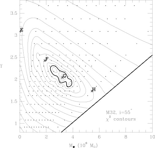
An example is given in Figure 2 which shows
 2 contours in
(Mh, M/L)-space
derived from ground-based and HST data for M32
([van der Marel et
al. 1998]).
The expected degeneracy appears as a plateau of nearly constant
2; this plateau
reflects the freedom to adjust
a three-integral f in response to changes in
such that
the goodness-of-fit to the data remains precisely unchanged.
When the potential is represented by just two parameters, this
non-uniqueness appears as a ridge line in parameter space, since
the virial theorem implies a unique relation between the two
parameters that define the potential
([Merritt 1994]).
Imperfections in the data or the modelling algorithm broaden this
ridge line into a plateau, often with spurious local minima.
The extreme degeneracy of models derived from such data means
that is usually impossible to learn much about the potential that
could not have been inferred from the virial theorem alone.
2 contours in
(Mh, M/L)-space
derived from ground-based and HST data for M32
([van der Marel et
al. 1998]).
The expected degeneracy appears as a plateau of nearly constant
2; this plateau
reflects the freedom to adjust
a three-integral f in response to changes in
such that
the goodness-of-fit to the data remains precisely unchanged.
When the potential is represented by just two parameters, this
non-uniqueness appears as a ridge line in parameter space, since
the virial theorem implies a unique relation between the two
parameters that define the potential
([Merritt 1994]).
Imperfections in the data or the modelling algorithm broaden this
ridge line into a plateau, often with spurious local minima.
The extreme degeneracy of models derived from such data means
that is usually impossible to learn much about the potential that
could not have been inferred from the virial theorem alone.
3.4. The Axisymmetric Inverse Problem
Modelling of elliptical galaxies has evolved in a very different way
from modelling of disk galaxies, where it was recognized early
on that most of the information about the mass distribution is contained
in the velocities, not in the light.
By contrast, most attempts at elliptical galaxy modelling have
used the luminosity as a guide to the mass, with the velocities
serving only to normalize the mass-to-light ratio.
One could imagine doing much better, going from the observed
velocities to a map of the gravitational potential.
The difficulties in such an "inverse problem" approach are
considerable, however.
The desired quantity, , appears
implicitly as a non-linear argument of f, which itself is unknown and
must be determined from the data.
There exist few uniqueness proofs that would even justify
searching for an optimal solution, much less
algorithms capable of finding those solutions.
A notable attempt was made by
Merrifield (1991),
who asked whether it was possible to infer a dependence of f on a
third integral in a model-independent way.
Merrifield pointed out that the velocity dispersions along either
the major or minor axes of an edge-on, two-integral axisymmetric
galaxy could be independently used to evaluate the kinetic energy
term in the virial theorem.
A discrepancy between the two estimates might be taken as
evidence for a dependence of f on a third integral.
Merrifield's test may be seen as a consequence of the fact that
f (E, Lz) is uniquely determined in an
axisymmetric galaxy with
known and
.
However, as Merrifield emphasized, a spatially varying M/L
could mimic the effects of a dependence of f on a third integral.
An algorithm for simultaneously recovering
f (E, Lz) and
(R, z) in an
edge-on galaxy, without any restrictions on the relative distribution of
mass and light, was presented by
Merritt (1996).
The technique requires complete information about the
rotational velocity and line-of-sight velocity dispersion
over the image of the galaxy.
One can then deproject the data to find unique expressions for
(R, z),
(R,
z) and ![]() (R, z).
Once these functions are known, the potential follows immediately
from either of the Jeans equations (25, 26);
f+(E, Lz) is
also uniquely determined, as described above.
The odd part of f is obtained from the
deprojected
(R, z).
Once these functions are known, the potential follows immediately
from either of the Jeans equations (25, 26);
f+(E, Lz) is
also uniquely determined, as described above.
The odd part of f is obtained from the
deprojected
![]() (R, z).
This work highlights the impossibility of ruling out
two-integral f's for axisymmetric galaxies based on observed
moments of the velocity distribution, since the potential can
always be adjusted in such a way as to reproduce the data without
forcing f to depend on a third integral.
(R, z).
This work highlights the impossibility of ruling out
two-integral f's for axisymmetric galaxies based on observed
moments of the velocity distribution, since the potential can
always be adjusted in such a way as to reproduce the data without
forcing f to depend on a third integral.
The algorithm just described may be seen as the generalization to
edge-on axisymmetric systems of algorithms that infer f
(E) and (r) in
spherical galaxies from the velocity dispersion profile (e. g.
[Gebhardt &
Fischer 1995]).
The spherical inverse problem is highly degenerate if
f is allowed to depend on L2 as well as
E (e.g.
[Dejonghe &
Merritt 1992]),
and one expects a similar degeneracy in the axisymmetric inverse problem
if f is allowed to depend on I3.
Thus the situation is even more discouraging than envisioned by
Fillmore & Levison
(1989),
who assumed that the data were restricted to the major or minor
axes: even knowledge of the velocity moments over the full image
of a galaxy is likely to be consistent with a large number of
(f,) pairs.
Distinguishing between these possible solutions clearly requires
additional information, and one possible source is line-of-sight velocity
distributions (LOSVD's), which are now routinely measured with
high precision
([Capaccioli &
Longo 1994]).
In the spherical geometry, LOSVD's have been shown to be
effective at distinguishing between different
f (E, L2) -
(R, z)
pairs that reproduce the velocity dispersion data equally well
([Merritt & Saha
1993];
[Gerhard 1993];
[Merritt 1993]).
A second possible source of information is proper
motions, which in the spherical geometry allow one to infer the
variation of velocity anisotropy with radius
([Leonard &
Merritt 1989]);
however most elliptical galaxies are too distant for
stellar proper motions to be easily measured.
A third candidate is X-ray gas, from which the potential can in
principle be mapped using the equation of hydrostatic equilibrium
([Sarazin 1988]).
All of the techniques described above begin from the assumption
that the luminosity distribution
(R, z) is known.
Rybicki (1986)
pointed out the remarkable fact that
is
uniquely constrained by the observed surface brightness
distribution of an axisymmetric galaxy
only if the galaxy is seen edge-on, or if some other
restrictive condition applies, e.g. if the isodensity contours
are assumed to be coaxial ellipsoids with known axis ratios.
Gerhard & Binney
(1996)
constructed axisymmetric density
components that are invisible when viewed in projection and
showed how the range of possible 's
increases as the inclination varies from edge-on to face-on.
Kochanek & Rybicki
(1996)
developed methods to produce families
of density components with arbitrary equatorial density
distributions; such components typically look like disks.
Romanowsky &
Kochanek (1997)
explored how uncertainties in
deprojected 's affect computed
values of the kinematical
quantities in two-integral models with constant mass-to-light ratios.
They found that large variations could be produced in the
meridional plane velocities but that the projected profiles were
generally much less affected.
These studies suggest that the dynamical inverse problem for axisymmetric galaxies is unlikely to have a unique solution except under fairly restrictive conditions. This fact is useful to keep in mind when evaluating axisymmetric modelling studies, in which conclusions about the preferred dynamical state of a galaxy are usually affected to some degree by restrictions placed on the models for reasons of computational convenience only.
1 Because of their boxlike shapes in the meridional plane, such orbits were originally called "boxes" even though their three-dimensional shapes are more similar to doughnuts. Back.