4. TRIAXIALITY

Motion in triaxial potentials differs in three important ways from motion in axisymmetric potentials. First, the lack of rotational symmetry means that no component of an orbit's angular momentum is conserved. While tube orbits that circulate about the symmetry axes still exist in triaxial potentials, other orbits are able to reverse their sense of rotation and approach arbitrarily closely to the center. The box orbits of Stäckel potentials are prototypical examples. Second, triaxial potentials are 3 DOF systems, and the objects that lend phase space its structure are the resonant tori that satisfy a condition between the three fundamental frequencies of the form l₁ + m₂ + n₃ = 0. Unlike the case of 2 DOF systems, where a resonance between two fundamental frequencies implies commensurability and hence closure, the resonant trajectories in 3 DOF systems are not generically closed; instead, they densely fill a thin, two-dimensional surface. Third, much of the phase space in realistic triaxial potentials is chaotic, particularly in models where the gravitational force rises rapidly toward the center.

The original motivation for studying triaxial models came from the observed slow rotation of elliptical galaxies ([Bertola & Capaccioli 1975]; [Illingworth 1977]), which effectively ruled out "isotropic oblate rotator" models. The low rotation could have been explained without invoking triaxiality, since any axisymmetric model can be made nonrotating by requiring equal numbers of stars to circulate in the two senses about the symmetry axis. But Binney (1978) argued that it was more natural to grant the existence of a global third integral, hence to assume that the flattening was due in part to anisotropy in the meridional plane. Binney argued further that two non-classical integrals were no less natural than one, and therefore that one might be able to build galaxies without rotational symmetry whose elongated shapes were supported primarily by the extra integrals. This suggestion was confirmed by Schwarzschild (1979, 1982) who showed that most of the orbits in triaxial potentials with large smooth cores do respect three integrals and that self-consistent triaxial models could be constructed by superposition of such orbits. Subsequent support for the triaxial hypothesis came from N-body simulations of collapse in which the final configurations were often found to be non-axisymmetric ([Wilkinson & James 1982]; [van Albada 1982]).

The case for triaxiality is perhaps less compelling now than it was ten or fifteen years ago. N-body simulations of galaxy formation that include a dissipative component often reveal an evolution to axisymmetry in the stars once the gas has begun to collect in the center ([Udry 1993]; [Dubinski 1994]; [Barnes & Hernquist 1996]). A central point mass, representing a nuclear black hole, has a similar effect ([Norman, May & van Albada 1985]; [Merritt & Quinlan 1998]). A plausible explanation for the evolution toward axisymmetry in these simulations is stochasticity of the box orbits resulting from the deepened central potential. Similar conclusions have been drawn from self-consistency studies of triaxial models with realistic, centrally-concentrated density profiles: the shortage of regular box orbits is often found to preclude a stationary triaxial solution ([Schwarzschild 1993]; [Merritt & Fridman 1996]; [Merritt 1997]). Observational studies of minor-axis rotation suggest that few if any elliptical galaxies are strongly triaxial ([Franx, Illingworth & de Zeeuw 1991]), and detailed modelling of a handful of nearby ellipticals, as discussed above, reveals that their kinematics can often be very well reproduced by assuming axisymmetry. The assumption that an oblate galaxy with counter-rotating stars would be unphysical has also been weakened by the discovery of a handful of such systems ([Rubin, Graham & Kenney 1992]; [Merrifield & Kuijken 1994]).

The phenomenon of triaxiality nevertheless remains a topic of vigorous study, for a number of reasons. At least some elliptical galaxies and bulges exhibit clear kinematical signatures of non-axisymmetry (e.g. [Schechter & Gunn 1979]; [Franx, Illingworth & Heckman 1989]), and the observed distribution of Hubble types is likewise inconsistent with the assumption that all ellipticals are precisely axisymmetric ([Tremblay & Merritt 1995], 1996; [Ryden 1996]). Departures from axisymmetry (possibly transient) are widely argued to be necessary for the rapid growth of nuclear black holes during the quasar epoch ([Shlosman, Begelman & Frank 1990]), for the fueling of starburst galaxies ([Sanders & Mirabel 1996]), and for the large radio luminosities of some ellipticals ([Bicknell et al. 1997]). These arguments suggest that most elliptical galaxies or bulges may have been triaxial at an earlier epoch, and perhaps that triaxiality is a recurrent phenomenon induced by mergers or other interactions.

Almost all of the work reviewed below deals with nonintegrable triaxial models. Integrable triaxial potentials do exist - the Perfect Ellipsoid is an example - but the integrable models always have features, like large, constant-density cores, that make them poor representations of real elliptical galaxies. More crucially, integrable potentials are "non-generic" in the sense that their phase space lacks many of the features that are universally present in non-integrable potentials. For instance, the box orbits in realistic triaxial potentials are strongly influenced by resonances between the three degrees of freedom, while in integrable potentials these resonances (although present) have no effect and all the box orbits belong to a single family. Integrable triaxial models are reviewed by de Zeeuw (1988) and Hunter (1995).

The standard convention is adopted here in which the long and short axes of a triaxial figure are identified with the x and z axes respectively.

4.1. The Structure of Phase Space

The motion in smooth triaxial potentials has many features in common with more general dynamical systems. Some relevant results from Hamiltonian dynamics are reviewed here before discussing their application to triaxial potentials.

Motion in non-integrable potentials is strongly influenced by resonances between the fundamental frequencies. A resonant torus is one for which the frequencies _i satisfy a relation n . = 0 with n = (l, m, n) an integer vector. Resonances are dense in the phase space of an integrable Hamiltonian, in the sense that every torus lies near to a torus satisfying n . = 0 for some (perhaps very large) integer vector n. However, most tori are very non-resonant in the sense that n . is large compared with |n|^{-(N + 1)}, with N the number of degrees of freedom. As one gradually perturbs a Hamiltonian away from integrable form, the KAM theorem guarantees that the very non-resonant tori will retain their topology, i.e. that the motion in their vicinity will remain quasiperiodic and confined to (slightly deformed) invariant tori. Resonant tori, on the other hand, can be strongly affected by even a small perturbation.

In a 2 DOF system, motion on a resonant torus is closed, since the resonance condition implies that the two frequencies are expressible as a ratio of integers, ₁ / ₂ = |m / l|. In three dimensions, a single relation n . = 0 between the three frequencies does not imply closure; instead, the trajectory is confined to a two-dimensional submanifold of its 3-torus. The orbit in configuration space lies on a thin sheet. (In the special case that one of the elements of n is zero, two of the frequencies will be commensurate.) For certain tori, two independent resonance conditions n . = 0 will apply; in this case, the fundamental frequencies can be written _i = n_{i 0}, i.e. there is commensurability for each frequency pair and the orbit is closed.

On a resonant torus in an integrable Hamiltonian, every trajectory satisfies the resonance conditions (of number K N - 1) regardless of its phase. Among this infinite set of resonant trajectories, only a finite number persist under perturbation of the Hamiltonian, as resonant tori of dimension N - K. The character of these remaining tori alternates from stable to unstable as one varies the phase around the original torus. Motion in the vicinity of a stable resonant torus is regular and characterized by N fundamental frequencies. Motion in the vicinity of an unstable torus is generically stochastic, even for small perturbations of the Hamiltonian. Furthermore, in the neighborhood of a stable resonant torus, higher-order resonances occur which lead to secondary regions of regular and stochastic motion, etc., down to finer and finer scales.

In a weakly perturbed Hamiltonian, the stochastic regions tend to be isolated and the associated orbits are often found to mimic regular orbits for many oscillations. ⁽²⁾ As the perturbation increases, the stochastic regions typically grow at the expense of the invariant tori. Eventually, stochastic regions associated with different unstable resonances overlap, producing large regions of phase space where the motion is interconnected. One often observes a sudden transition to large-scale or "global" stochasticity as some perturbation parameter is varied. In a globally stochastic part of phase space, different orbits are effectively indistinguishable and wander in a few oscillations over the entire connected region. Such orbits rapidly visit the entire configuration space region within the equipotential surface, giving them a time-averaged shape that is approximately spherical.

The way in which resonances affect the phase space structure of nonrotating triaxial potentials has recently been clarified by a number of studies ([Carpintero & Aguilar 1998]; [Papaphilippou & Laskar 1998]; [Valluri & Merritt 1998]) that used trajectory-following algorithms to extract the fundamental frequencies and to identify stochastic orbits. The discussion that follows is based on this work and on the earlier studies of Levison & Richstone (1987), Schwarzschild (1993) and Merritt & Fridman (1996).

At a fixed energy, the phase space of a triaxial galaxy is five-dimensional. One expects most of the regular orbits to be recoverable by varying the initial conditions over a space of lower dimensionality; for instance, in an integrable potential, all the orbits at a given energy can be specified via the 2D set of actions. Levison & Richstone (1987) advocated a 4D initial condition space consisting of coordinates (x₀, z₀, y₀ = 0) and velocities (₀, ₀), with ₀ determined by the energy. Schwarzschild (1993) argued that most orbits could be recovered from just two, 2D initial condition spaces. His first space consisted of initial conditions with zero velocity on one octant of the equipotential surface; these initial conditions generate box orbits in Stäckel potentials. The second space consisted of initial conditions in the (x, z) plane with ₀ = ₀ = 0 and ₀ determined by the energy. This space generates the four families of tube orbits in Stäckel potentials. Papaphilippou & Laskar (1998) suggested that boxlike orbits could be generated more simply by setting all coordinates to zero and varying the two velocity components parallel to a principal plane. This choice for box-orbit initial condition space is not precisely equivalent to Schwarzschild's; it excludes resonant orbits (e.g. the banana) that avoid the center, while Schwarzschild's excludes orbits (e.g. the anti-banana) that have no stationary point.

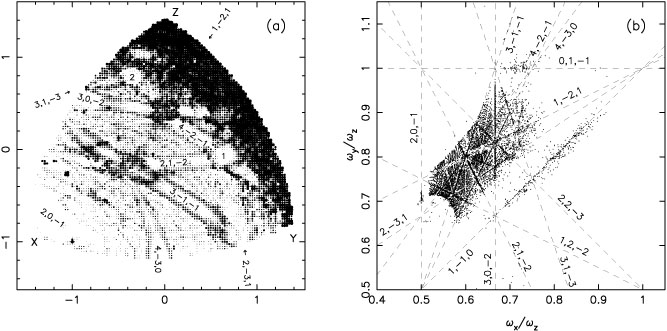
Figure 3a illustrates stationary (box-orbit) initial condition space at one energy in a triaxial Dehnen model with c/a = 0.5, b/a = 0.79 and = 0.5, a "weak cusp." The figure was constructed from ~ 10⁴ orbits with starting points lying on the equipotential surface; the greyscale was adjusted in proportion to the logarithm of the stochasticity, measured via the rate of diffusion in frequency space. Initial conditions associated with regular orbits are white. Figure 3b shows the frequency map defined by the same orbits, i.e. the ratios _x / _z and _y / _z between the fundamental frequencies associated with motion along the three coordinate axes. The most important resonances, l_x + m_y + n_z = 0, are indicated by lines in the frequency map and by their integer components (l, m, n) in Figure 3a. Intersections of these lines correspond to closed orbits, _i = n_{i 0}. In order to keep the frequency map relatively simple, all orbits associated with a stable resonance have been plotted precisely on the resonance line; the third fundamental frequency (associated with slow rotation around the resonance) has been ignored. Unstable resonances appear as gaps in the frequency map, since the associated orbits do not have well-defined frequencies.

Figure 3. Box-orbit phase space at roughly the half-mass energy in a triaxial Dehnen model with cusp slope = 0.5 (Valluri & Merritt 1998). (a) Initial condition space: one octant of the equipotential surface has been projected onto a plane. Each orbit begins on this surface with zero velocity. The top, left and right corners correspond to the z (short), x (long) and y (intermediate) axes. The grey scale is proportional to the logarithm of the diffusion rate of orbits in frequency space; initial conditions corresponding to regular orbits are white. The regions labelled "1" and "2" are starting points associated with the 5 : 6 : 8 and 7 : 9 : 10 periodic orbits, respectively. Other regions are labelled with the integers (l, m, n) that define resonance zones. (b) Frequency map: the fundamental frequencies are plotted as ratios x / z and y / z for each of the orbits in (a). The most important resonances are labelled. Stable resonances produce solid lines; gaps correspond to unstable (chaotic) resonances.

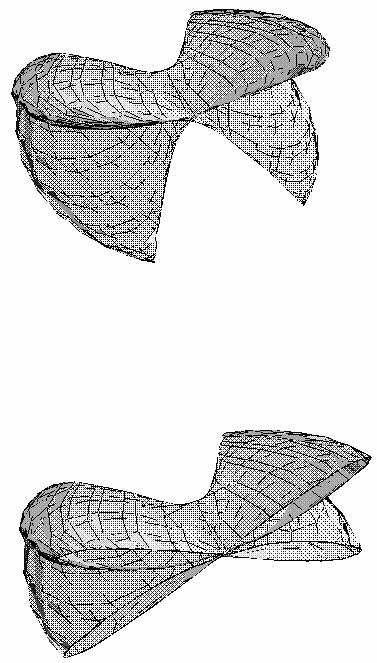
Following the discussion above, one expects the regular orbits to come in three families corresponding to the number K = (0, 1, 2) of independent resonance conditions that define their associated phase space regions. The three families are in fact apparent in Figure 3. First are the regular orbits that lie in the regions between the resonance zones, K = 0. Orbits in these regions are regular for the same reason that box orbits in a Stäckel potential are regular, i.e. because the region of phase space in which they are located is locally integrable. ⁽³⁾ In configuration space, these orbits densely fill a three-dimensional region centered on the orgin. A second set of regular orbits lie in zones associated with a single resonance, K = 1; examples are the (2, 1, - 2), (3, - 1, - 1) and (4, - 2, - 1) resonance zones. The stable resonant orbits that define these regions are "thin boxes" that fill a sheet in configuration space (Figure 4); the regular orbits around them have a small but finite thickness. The planar x - z banana (2, 0, - 1) and fish (3, 0, - 2), and the x - y pretzel (4, - 3, 0), also generate families of thin orbits. The third set of regular orbits, the "boxlets," surround periodic orbits that lie at the intersection of two resonances, K = 2. Two such regions are apparent in Figure 3a, associated with the 5 : 6 : 8 and 7 : 9 : 10 periodic orbits (marked 1 and 2).

Figure 4. A thin box orbit associated with the (2, 1, - 2) resonance in Figure 3. The lower view is a cutaway showing that the orbit is confined to a membrane.

Close inspection of Figure 3a suggests that even the "integrable" (K = 0) regions are threaded with high-order resonances and their associated chaotic zones. One expects to find such structure since resonant tori are dense in the phase space of the unperturbed Hamiltonian. However the stochasticity associated with the high-order resonances is very weak and for practical purposes the orbits in these regions are regular throughout.

All of the box orbits in a Stäckel potential belong to a single family with smoothly varying actions. While resonances like those shown in Figure 3 are present in Stäckel potentials, their effect on the motion is limited to the resonant tori themselves. By contrast, in the phase space of tube orbits, even Stäckel potentials contain (up to) three important resonances at each energy corresponding to the three families of thin tube orbits. These primary resonances persist in nonintegrable potentials and generate families of regular tube orbits similar to those in Stäckel potentials. The transition zones between the various tube orbit families, which are occupied by unstable orbits in a Stäckel potential, are now stochastic, although the stochastic zones are typically narrow. Valluri & Merritt (1998) illustrated the time evolution of a stochastic tube orbit.

The structure in Figure 3 is characteristic of mildly non-integrable triaxial potentials. As the perturbation of the potential away from integrability increases - due to an increasing central density, for instance - the parts of phase space corresponding to tube orbits are only moderately affected. However the boxlike orbits are sensitively dependent on the form of the potential near the center. Papaphilippou & Laskar (1998) studied ensembles of orbits in the logarithmic triaxial potential at fixed energy; they took as their perturbation parameter the axis ratios of the model. At extreme elongations, high-order resonances became important in box-orbit phase space; for instance, in a triaxial model with c/a = 0.18, significant stochastic regions associated with the (3, - 1, 0) and (6, - 1, - 1) resonances were found. Valluri & Merritt (1998) varied the cusp slope and the mass of a central black hole in a family of triaxial Dehnen models. They found that the relative contributions from the three types of regular orbit (satisfying 0, 1, or 2 resonance conditions) in box-orbit phase space shifted as the perturbation increased, from K = 0 (box orbits) at small perturbations, to K = 1 (thin boxes) at moderate perturbations, to K = 2 (boxlets) at large perturbations.

4.2. Periodic Orbits

As discussed above, the objects that give phase space its structure in 3 DOF systems are the resonant tori which satisfy a condition l₁ + m₂ + n₃ = 0 between the three fundamental frequencies. The corresponding orbits are thin tubes or thin boxes. However most studies of the motion in triaxial potentials have focussed on the principal planes, in which resonances (i.e. l₁ + m₂ = 0) are equivalent to closed orbits. Figure 3a suggests that most of the regular orbits in a triaxial potential are associated with thin orbits rather than with closed orbits. The closed orbits are nevertheless worth studying for a number of reasons. Gas streamlines must be non-self-intersecting, which restricts the motion of gas clouds to closed orbits like the 1 : 1 loops. Elongated boxlets like the bananas have shapes that make them very useful for reproducing a barlike mass distribution, and one expects such orbits to be heavily populated in self-consistent models. The fraction of regular orbits associated with closed orbits (as opposed to thin orbits) also tends to increase as the phase space becomes more and more chaotic, as discussed below.

4.2.1. Nonrotating Potentials

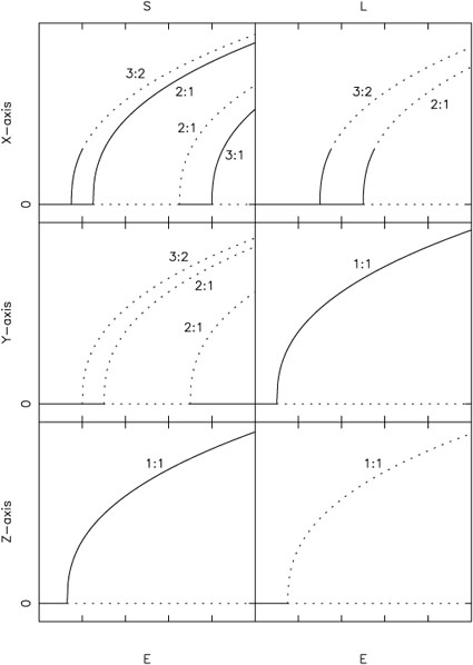
Periodic orbits in the principal planes of triaxial models often first appear as bifurcations from the axial orbits. Figure 5 is a representative bifurcation diagram for axial orbits in nonrotating triaxial models with finite central forces, based on the studies of Heiligman & Schwarzschild (1979), Goodman & Schwarzschild (1981), Magnenat (1982a), Binney (1982a), Merritt & de Zeeuw (1983), Miralda-Escudé & Schwarzschild (1989), Pfenniger & de Zeeuw (1989), Lees & Schwarzschild (1992), Papaphilippou & Laskar (1996, 1998), and Fridman & Merritt (1997). When the central force is strongly divergent, as would be the case in a galaxy with a central black hole, the axial orbits are unstable at all energies but many of the other periodic orbits in Figure 5 still exist.

Figure 5. Representative bifurcation diagram for planar periodic orbits in non-axisymmetric potentials with finite central forces. The three rows show bifurcations from the x (long), y (intermediate) and z (short) axes. The left column (S) shows bifurcations in the plane containing the shorter of the two remaining axes, while the right column (L) shows bifurcations in the plane containing the longer axis. Solid lines correspond to stable orbits and dotted lines to unstable orbits, where stability is defined with respect to motion in the appropriate plane.

The x-axis orbit does not experience a 1 : 1 bifurcation since its frequency is always less than that of perturbations along either of the two shorter axes. However at sufficiently high energies, the x oscillation frequency falls to 1/2 the frequency of a z perturbation and the 2 : 1 x - z banana orbit appears (Figure 6). At still higher energies, a second 2 : 1 bifurcation produces the x - y banana; following this bifurcation, the x-axis orbit is typically unstable in both directions. This second bifurcation occurs most readily in nearly prolate models where the y and z axes are nearly equal in length. The energy of the first, x - z bifurcation is a strong function of the degree of central concentration of the model, as measured for instance by the cusp-slope parameter in Dehnen's model. For 1, the x-axis orbit is unstable at most energies in all but the roundest triaxial models.

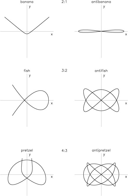
Figure 6. Resonant box orbits in a principal plane of a triaxial potential. Left: centrophobic boxlets; these are typically stable. Right: centrophilic boxlets; these are typically unstable.

In highly elongated models, c/a 0.45, the x axis orbit can return to stability at the bifurcation of the "antibanana" orbit, a 2 : 1 resonant orbit that passes through the center (Figure 6). Miralda-Escudé & Schwarzschild (1989) call such orbits "centrophilic;" resonant orbits that avoid the center, like the x - z banana, are "centrophobic." In nearly oblate models, this return to stability in the x - z plane causes the x-axis orbit to become stable in both directions. The x-axis orbit can become unstable once more at still higher energies when c/a is sufficiently small, through the appearance of a 3 : 1 resonance in the direction of the z axis.

Both the y- and z-axis orbits are unstable at all energies above the 1 : 1 bifurcations. The y-axis orbit can become unstable in both directions following the 2 : 1 bifurcation that produces the y - z banana. In highly elongated models, the y-axis orbit returns briefly to stability in the z-direction through the appearance of the y - z anti-banana.

Additional bifurcations of the form n : m, with both n and m greater than one, can occur from the axial orbits. These bifurcations typically do not affect the stability of the axial orbits but they are nevertheless important because they generate additional families of periodic orbits. The name "boxlet" was coined by Miralda-Escudé & Schwarzschild (1989) for these orbits (Figure 6). The 3 : 2 boxlets are "fish," the 4 : 3 boxlets are "pretzels," etc. Only the fish orbits have been extensively studied; they first appear as 3 : 2 bifurcations from the x-axis orbit (x - z and x - y fish) or the y-axis orbit (y - z fish), typically at energies below the banana bifurcation. The x - y fish is only important in highly prolate models.

The boxlets can themselves become unstable, either to perturbations in the plane of the orbit or to vertical perturbations. The x - z banana exists and is stable over a wide range of model parameters; it becomes unstable only in nearly prolate models, through a vertical 2 : 1 bifurcation. The x - y and y - z bananas are usually vertically unstable; the x - y banana returns to stability only in highly elongated, nearly prolate models. In nearly oblate models, the x - z fish first becomes unstable to perturbations in the orbital plane, while for strongly triaxial and prolate models instability first appears in the vertical (y) direction. The x - y fish is only important in strongly prolate models; in strongly triaxial or oblate models, it either does not exist, or is generally unstable to vertical perturbations. The y - z fish is almost always vertically unstable.

As the central concentration of a triaxial model increases, the axial orbits become unstable over a progressively wider range of energies. In models with steep central cusps or central black holes, the axial orbits are unstable at all energies and the (centrophobic) boxlets may extend all the way to the center. Little systematic work has been done on the properties of boxlets in such models. Miralda-Escudé & Schwarzschild (1989) investigated the orbit structure in the principal planes of two triaxial models with = log(R_c² + m²) as R_c was varied; for R_c = 0, their models have an r^-2 central density cusp. Miralda-Escudé & Schwarzschild found that the lowest-order boxlets continued to exist, typically with no change in their stability properties, as R_c was reduced to zero. The centrophobic boxlets were also found to be not strongly affected by the addition of a central point mass. Pfenniger & de Zeeuw (1989) investigated the banana boxlets in a second family of models with = 2 cusps. They found that the bananas became strongly bent for model axis ratios c/a 0.65, making them less useful for reconstructing the model shape. In their survey of orbits in two triaxial models with Dehnen's density law, Merritt & Fridman (1996) found that the x - z fish was vertically unstable at most energies for = 1 and at all energies for = 2. Only the x - z fish, of all the planar boxlet families, remained stable over an appreciable energy range in the two models investigated by them. A number of higher-order resonances outside of the principal planes were also found to be important, including the 4 : 5 : 7, 5 : 6 : 8 and 6 : 7 : 9 boxlets.

4.2.2. Rotating Models

A great deal of work has been done on periodic orbits in models of barred galaxies ([Contopoulos & Grosbøl 1989]; [Sellwood & Wilkinson 1993]). Most of this work has been restricted to motion in the equatorial plane; furthermore, models of barred galaxies typically have low central concentrations, mild departures from axisymmetry ("weak bars"), and rapid rotation, making them poor representations of elliptical galaxies. The smaller number of studies of periodic orbits in rotating elliptical galaxy models have focussed on two low-order resonant families: the 1 : 1 orbits that bifurcate from the axial orbits, giving rise to the tubes; and the 1 : 2 banana orbits.

An early study of the closed orbits in Schwarzschild's (1979) triaxial model ([Merritt 1979]) revealed that the 1 : 1 orbits circling the long axis continue to exist when the figure rotates, but are tipped by the Coriolis force out of the y - z plane. The tip angle increases with energy and the family terminates when it mergers with the retrograde closed orbits in the equatorial plane. Heisler, Merritt & Schwarzschild (1982) called these tipped orbits "anomalous" and noted the existence of a second, unstable family of anomalous orbits circling the intermediate axis. A large number of additional studies have traced the existence and stability of these orbits in a variety of rotating triaxial potentials ([Binney 1981]; [Tohline & Durisen 1982]; [Magnenat 1982a], b; [de Zeeuw & Merritt 1983]; [Durisen et al. 1983]; [Merritt & de Zeeuw 1983]; [Mulder 1983]; [Mulder & Hooimeyer 1984]; [Martinet & de Zeeuw 1988]; [Cleary 1989]; [Patsis & Zachilas 1990]; [Hasan, Pfenniger & Norman 1993]). One motivation for this work has been the expectation that gas or dust falling into a rotating triaxial galaxy might dissipatively settle onto the anomalous orbits before finding its way into the center ([Tohline & Durisen 1982]; [van Albada, Kotanyi & Schwarzschild 1982]).

The existence of the anomalous orbits is tied to the vertical instability of the orbits in the equatorial plane. There are four major families of planar orbits: two of these (the "x₁" and "x₄" families in Contopoulos's convention), both prograde, remain close to the x and y axes respectively; the other two (x₂ and x₃) are prograde and retrograde counterparts of the 1 : 1 orbit that bifurcates from the y axis in nonrotating models. One of these - either the retrograde orbit, if figure rotation is about the short axis, or the prograde orbit, if rotation is about the long axis - is unstable to perturbations out of the plane of rotation over a wide radial range. In either case, a family of anomalous orbits exists that is inclined to the plane of rotation; the family has two branches that are tipped in opposite directions with respect to the equatorial plane but which circle the short axis in the same sense. The anomalous orbits first appear at low energies as 1 : 1 bifurcations of the z - axis orbit. In models without cores, the z-axis orbit may be unstable at all energies and the anomalous orbits extend into the center. In models with sufficiently high rotation, on the other hand, the anomalous orbits can bifurcate twice from the family in the plane, never reaching the z-axis. The unstable anomalous orbits that circle the intermediate axis first appear at the bifurcation of the 1 : 1 orbit in the x - z plane.

Miller & Smith (1979) investigated the motion of particles in a 3D, rotating N-body bar. They found that nearly half of the orbits could be described as respecting a 2 : 1 resonance between the x and z motions. Pfenniger & Friedli (1991) likewise found a large population of 2 : 1 orbits in their rotating N-body models. This family of orbits, which reduces to the x - z bananas in the case of zero figure rotation, has been studied by a number of other authors including Mulder & Hooimeyer (1984), Cleary (1989), Martinet & Udry (1990), Patsis & Zachilas (1990), Udry (1991), and Hasan, Pfenniger & Norman (1993). The family bifurcates from the prograde x₁ family at low energies and so retains the x - y commensurability of that orbit - either 1 : 1 (low energies) or 3 : 1 (high energies). The radial range over which it exists decreases with increasing rotation of the figure. At large energies, the x₁ orbit returns to vertical stability through bifurcation of the x - z anti-banana. At even greater energies, both banana families may merge again with the x₁ orbits. Udry (1991) traced the existence and stability of the 2 : 1 orbits that bifurcate from the y and z axes and from the other 1 : 1 families in the equatorial plane. None of these families is likely to be as important as the x - z bananas in self-consistent models.

4.3. Stochasticity

4.3.1. Origin

Stochasticity always occurs near an unstable resonant torus. Such tori exist and are dense even in integrable systems, but the motion in their vicinity is (by definition) regular; under perturbation of the potential, however, resonant tori are destroyed and the motion undergoes a qualitative change. The reason for this change is suggested by Figure 7, which shows an orbit that lies close to the short- (y-) axis orbit in the potential of a 2D bar. Such an orbit can be represented as the superposition of a rapid radial oscillation and a slow angular rotation, with frequencies _r and respectively; tends to zero as the orbit approaches the axial orbit. Resonances between the fast and slow motions satisfy a condition l - m_r = 0. As tends to zero, the separation between neighboring resonances, defined by l and l + 1, also becomes small, resulting in motion that is extremely complex. In fact one can show that the motion is generically no longer confined to tori; instead the trajectory moves more-or-less randomly through a region of dimensionality 2N - 1, where N is the number of degrees of freedom. Among the properties of the motion in these stochastic regions is exponential divergence of initially close trajectories ([Miller 1964]; [Oseledec 1968]), resulting in extreme sensitivity to small changes in the initial conditions.

Figure 7. An orbit that lies close to the unstable, short- (y-) axis orbit in a 2D barred potential. The motion consists of a rapid radial oscillation combined with a slow rotation. Resonances between the fast and slow motions produce a stochastic zone where the motion is exponentially unstable.

An early indication of the importance of stochasticity in triaxial potentials was the discovery that some of the orbits in Schwarzschild's (1979) triaxial model yielded different occupation numbers when integrated using a different computer ([Merritt 1980]), a consequence of the exponential divergence just mentioned. Goodman & Schwarzschild (1981) computed rates of divergence between pairs of box-orbit trajectories at one energy in this potential; they found that about a fourth of the orbits were stochastic. Most of the unstable orbits had their starting points near the z axis, producing a narrow strip of instability in initial condition space; a similar stochastic strip can be seen in Figure 3a. Goodman & Schwarzschild showed that both the y and z axis orbits were linearly unstable at this energy while the x axis orbit was stable. They speculated that the stochasticity was connected with this instability; in particular, they noted that the z-axis orbit was strongly unstable to perturbations in both directions, following the bifurcation of the 1 : 1 loop orbits in the y - z and x - z planes.

The stochasticity of the motion near the short axis orbit (as opposed to the instability of the axial orbit, a weaker condition) was established by Gerhard (1985) using a method due to Melnikov (1963). Melnikov's method is based on the qualitative change that occurs in the shape of the phase curve, or "separatrix," of an unstable 2D orbit in the surface of section when the motion in its vicinity becomes stochastic. In a two-dimensional integrable potential, the separatrix is a smooth curve that intersects itself at the fixed ("homoclinic") point corresponding to an unstable orbit like the one in Figure 7. Under perturbation, the two branches of the separatrix corresponding to motion toward and away from the fixed point need not join smoothly; instead they can oscillate wildly, producing an infinite set of additional homoclinic points. The stochasticity may be interpreted as a consequence of this complex behavior. Melnikov defined an integral quantity that measures the infinitesimal separation between the two branches of the separatrix that approach and depart from the unstable fixed point. If this distance changes sign as one proceeds around the separatrix, nonintegrability has been rigorously established. Gerhard took as his integrable potential a 2D Stäckel model in which the total density fell off as r^-2 and the non-axisymmetric component as r^-4. He showed that certain perturbations, e.g. density terms varying as cos(m) with m odd, produced a rapid breakdown in the regularity of the motion near the short-axis orbit.

Martinet & Udry (1990) noted that most of the stochasticity in slowly-rotating planar models appeared to be associated with the x₃ family, which reduces to the unstable short-axis orbit in the limit of zero rotation. They traced the interactions of higher-order resonances in the vicinity of the x₃ orbit and argued that the development of a large stochastic layer in the surface of section could be attributed to the simultaneous action of these resonances. Martinet & Udry found that the stochastic region associated with this orbit tended to contract as the rate of figure rotation increased.

The 1 : 1 bifurcation that first induces instability in the z-axis orbit occurs at lower and lower energies as the central concentration of a triaxial model is increased. At the same time, the sensitivity of the axial orbits to small perturbations increases as the central force steepens. These two facts imply a greater role for stochasticity in triaxial models with high central densities. ⁽⁴⁾ Gerhard & Binney (1985) investigated 2 DOF motion in a bar with a central density cusp, ~ r^-, or a central point mass M_h representing a supermassive black hole. Using surfaces of section, they found that the fraction of phase space associated with stochastic motion increased with increasing or M_h. However, regular boxlike orbits persisted in families associated with low-order resonances like the 2 : 1 banana. Miralda-Escudé & Schwarzschild (1989) studied the orbits in a planar logarithmic potential as a function of core radius R_c. Even for R_c = 0, corresponding to a ~ r^-2 density cusp, the stochastic regions were found to be confined to narrow filaments in the surface of section between the resonant families. Papaphilippou & Laskar (1996) likewise found only a modest degree of stochasticity in their study of 2D logarithmic potentials with cores. Touma & Tremaine (1997) obtained similar results in the planar logarithmic potential using an approximate mapping technique.

Studies like these of 2 DOF motion tend to underestimate the importance of stochasticity in triaxial potentials, for at least three reasons. Periodic orbits that generate families of regular trajectories in the principal planes are often unstable to perturbations out of the plane; examples are the x - y and y - z bananas discussed above. Second, there are unstable periodic orbits that exist outside of the principal planes; some examples can be seen in Figure 3. Third, much of the stochasticity in 3 DOF systems is associated with resonances between the three degrees of freedom which have no analog in 2 DOF systems.

Techniques like surfaces of section that work well in 2 DOF systems can become cumbersome in three dimensions. An alternative technique for identifying an orbit as stochastic is to compute its Liapunov exponents, the mean exponential rates of divergence of a set of trajectories surrounding it. In a 3 DOF system there are six Liapunov exponents for every trajectory, corresponding to the six dimensions of phase space; the exponents come in pairs of opposite sign, a consequence of the conservation of phase space volume. Of the three independent exponents, one - corresponding to displacements in the direction of the motion - is always zero. The two remaining exponents, ₁ and ₂, may be seen as defining the time-averaged divergence rates in two directions orthogonal to the trajectory. For a regular orbit, ₁ = ₂ = 0; for a stochastic orbit, at least one (and typically two) of these exponents is nonzero.

Udry & Pfenniger (1988) computed all six Liapunov exponents for ensembles of orbits in triaxial potentials based on a modified Hubble law, which has a constant-density core and a large-radius density dependence of r^-3. To this model they added perturbing forces of various kinds, corresponding to central mass concentrations and angular distortions of the density. Udry & Pfenniger presented their results in terms of histograms of Liapunov exponents without distinguishing between different types of orbit or between orbits of different energies. Nevertheless they found that the average degree of stochasticity for a given potential always increased with increasing strength of the perturbation. Schwarzschild (1993) computed the largest Liapunov exponent for the orbits in his scale-free, r^-2 triaxial models discussed below. He found that most of the boxlike orbits, and a modest but significant fraction of the tube orbits, were stochastic; the y - z instability strip first discussed by Goodman & Schwarzschild (1981) was typically greatly enlarged in the scale-free models. Merritt & Fridman (1996) demonstrated that the boxlike orbits in a triaxial model with a cusp as shallow as ~ r^-1 were also mostly stochastic, though many of these orbits mimicked regular orbits for tens or hundreds of orbital periods. They noted that much of the stochasticity was generated by resonances not associated with the z-axis orbit. Merritt & Valluri (1996) showed that the histogram of Liapunov exponents of box orbits at a given energy tended toward a narrow spike as the integration time increased, consistent with the expectation that the stochastic parts of phase space are interconnected via the Arnold web. They found that both ₁ and ₂ were significantly nonzero for all of their orbits, suggesting that no isolating integrals existed aside from the energy.

4.3.2. Transition to Global Stochasticity

The KAM theorem guarantees that motion in the vicinity of a "very nonresonant" torus in an integrable system will remain regular under small perturbations of the potential. Since the majority of tori are very nonresonant - in the sense that rational numbers are rare compared to irrational ones - the KAM theorem says that a small perturbation of an integrable potential will leave most of the trajectories regular. At the same time, the resonant tori are dense in the phase space, and even an infinitesimal perturbation can cause the motion in their vicinity to become chaotic. When the perturbation is small, these chaotic regions are narrow and the motion within them tends to mimic regular motion for many oscillations. As the perturbation is increased, the chaotic zones from different resonant tori become wider and neighboring zones begin to overlap. Eventually one expects to find large regions of interconnected phase space where the motion is fully stochastic ([Hénon & Heiles 1964]).

The studies summarized above suggest that the behavior of box orbits in triaxial potentials can be strongly influenced by the steepness of the central force law, and it is natural to ask how centrally concentrated a triaxial model must be before the parts of phase space associated with boxlike orbits become globally stochastic. Valluri & Merritt (1998) investigated this question in triaxial Dehnen models, taking as their perturbation parameters the slope of the central density cusp and the mass M_h of a central point representing a nuclear black hole. They measured stochasticity via the change of the fundamental frequencies of an orbit computed over a fixed interval of time; for a regular orbit = 0, while for a stochastic orbit the "fundamental frequencies" gradually change with time ([Laskar 1993]). A quantity like is a more useful diagnostic of stochasticity than the Liapunov exponents since it measures a finite, rather than infinitesimal, displacement of an orbit due to stochastic diffusion. Valluri & Merritt found a fairly well-defined transition to global stochasticity in the phase space of boxlike orbits as M_h increased past ~ 2% of the galaxy mass (Figure 8). In models without a central point mass, the transition appeared to begin when the central cusp slope reached ~ 2, close to the largest value seen in real galaxies. Valluri & Merritt constructed histograms of diffusion rates in frequency space and found that weakly chaotic potentials exhibited a ~ 1 / distribution, extending over at least six decades in . As M_h or was increased, this distribution flattened, although every model investigated by them contained a significant number of slowly-diffusing stochastic orbits. Valluri & Merritt estimated that stochastic orbits would induce significant changes in the shape of a triaxial galaxy over its lifetime if 2, or if M_h exceed ~ 0.5% times the galaxy mass.

Figure 8. Transition to global stochasticity in stationary (box-orbit) initial condition space (Valluri & Merritt 1998). Each frame shows an octant of the equipotential surface, at roughly the half-mass radius, in a triaxial Dehnen model with = 0.5 and with a central point containing a fraction Mh of the total mass of the model. The z- (short) axis is vertical and the x- (long) axis is to the left. The grey scale is proportional to the logarithm of the diffusion rate in frequency space; white regions correspond to regular orbits. When Mh > 0.02, the motion is essentially fully stochastic at this energy.

Papaphilippou & Laskar (1998) used the same technique to compute diffusion rates in frequency space for ensembles of orbits in the logarithmic triaxial potential. They chose a fixed energy and core radius R_c such that the maximum amplitude of the motion was approximately 8R_c; as perturbation parameters they chose the axis ratios of the model. They found a striking increase in the diffusion rates of boxlike orbits in frequency space as the models became flatter.

4.4. Self-Consistent Models

Following Schwarzschild (1979, 1982), a standard technique for constructing stationary triaxial models has been to integrate large numbers of orbits for ~ 10² periods, store their time-averaged densities in a set of cells, and then reproduce the known mass of the model in each cell via orbital superposition. The technique is best suited to integrable potentials in which time-averaged densities correspond to uniformly populated tori ([Vandervoort 1984]; [Statler 1987]). In non-integrable potentials, a decision must be made about how to populate the stochastic parts of phase space. At one extreme, if stochastic diffusion rates are high, it is appropriate to assume that the stochastic parts of phase space at each energy are uniformly populated. In a weakly chaotic potential, on the other hand, stochastic orbits should be treated more like regular orbits since they remain confined to restricted regions of phase space over astronomically interesting time scales. Since orbits with a wide variety of shapes are useful for reproducing the density of a triaxial model, one expects the range of self-consistent solutions to be strongly dependent on how much of phase space is stochastic and on how the stochastic orbits are treated.

Schwarzschild (1979, 1982) emphasized the regular appearance of most of the orbits in his modified Hubble model, a consequence of its relatively low degree of central concentration. He found that self-consistency required appreciable numbers of orbits from both the box and tube families, a conclusion reached also by Statler (1987) who constructed models based on the Perfect Ellipsoid. The most strongly triaxial models in Statler's survey were dominated by box orbits; tube orbits appeared in significant numbers only when the geometry was favorable, i.e. when the figure was nearly oblate or prolate. Levison & Richstone (1987) likewise found a predominance of regular or nearly-regular orbits in their model-building study based on the logarithmic potential with a finite-density core. Levison & Richstone noted that many of the box orbits failed to exhibit reflection symmetry, a likely indication that they were associated with resonances.

Kuijken (1993) carried out a self-consistency study of scale-free, non-axisymmetric disks. His models had a surface density

(32)

with n = 2 or 4; the asymptotic dependence is r^-1, corresponding to a logarithmic density law, and the parameter n fixes the shapes of the isodensity contours, which are elliptical for n = 2 and become more boxy with increasing n. Kuijken found, in agreement with the earlier studies discussed above, that the 2D motion in triaxial potentials was mostly regular; however almost all of the boxlike orbits could be identified with one of the low-order resonant boxlets in Figure 6. He found that only axis ratios q 0.7 could be self-consistently reproduced for n = 2, and setting n = 4 restricted the allowed range of shapes even more. Syer & Zhao (1998) carried out a study similar to Kuijken's based on the scale-free disk models of Sridhar & Touma (1997), which have (R, ) = R^-1 S() for 0 1. The shape function S() in Sridhar & Touma's models is determined, for a given , by the requirement that the motion be fully regular; the corresponding models are peanut-shaped and highly elongated, with short-to-long axis ratios of ~ 1/3. Syer & Zhao found that no choice of the parameter permitted a self-consistent solution, a result which they ascribed to the restricted range of shapes of the boxlike orbits.

Schwarzschild (1993) carried out a study similar to Kuijken's in three dimensions. He chose the scale-free logarithmic potential with six different values for the axis ratios of the figure, from nearly oblate to nearly prolate; four of these were highly flattened. Stochasticity was identified via the largest Liapunov exponent ₁; as discussed above, a large fraction of the boxlike orbits were found to be stochastic in all of the model potentials. Schwarzschild was able to find self-consistent equilibria for each of his six models when all the orbits - both regular and stochastic - were included. In these models, the stochastic orbits were treated precisely like regular orbits, i.e. each was assigned a unique distribution of mass defined as the population of a set of grid cells averaged over ~ 50 orbital periods. When the stochastic orbits were excluded, only the rounder models could be reconstructed. Schwarzschild then estimated how rapidly the shapes of the models containing stochastic orbits would change due to their non-uniform population of phase space. He re-integrated the stochastic orbits for three times the interval of the original integration and recorded the change in their spatial distribution. This evolution was found to result in modest but significant changes in the overall shapes of the models.

Schwarzschild's scale-free models were designed to represent galactic halos, regions of low stellar density where a typical star will complete only a few tens of oscillations over the age of the universe. Closer to the centers of elliptical galaxies, orbital periods fall to 1% or less of a galaxy lifetime; since the rates of stochastic diffusion scale approximately with orbital frequencies, one expects the central parts of a triaxial galaxy to be much more strongly affected by stochasticity than the outer parts. Merritt & Fridman (1996) investigated the self-consistency of non-scale-free triaxial models obeying Dehnen's density law with = 1 ("weak cusp") and = 2 ("strong cusp") and c/a = 0.5. Treating the stochastic orbits like regular orbits yielded self-consistent solutions for both models; the regular orbits alone failed to reproduce either mass model. Merritt & Fridman then attempted to construct more nearly stationary solutions in which the stochastic parts of phase space were populated in a uniform way, especially at low energies, by combining all of the stochastic orbits at a given energy into a single ensemble. They found that no significant fraction of the mass could be placed on these "fully mixed" orbits in the strong-cusp model. Merritt (1997) extended this study to strong-cusp models with a range of shapes. He found (Figure 9) that only fairly oblate, prolate or spherical models could be constructed using the regular orbits alone.

Figure 9. Allowed axis ratios for self-consistent triaxial models with Dehnen's density law and = 2, a "strong cusp" (Merritt 1997). Only regular orbits were allowed in the solutions. The dotted curve denotes the approximate limit of solution space; points below correspond to models for which no self-consistent solution was found. Since many of the boxlike orbits in these models are stochastic, and since box orbits are necessary for maintaining triaxial figures, only nearly oblate and prolate solutions were found.

² Strictly speaking, the different stochastic regions in a 3 DOF system are always interconnected, but the time scale for diffusion from one such region to another (Arnold diffusion) is very long if the potential is close to integrable. Back.

³ The regularity of the box orbits in Stäckel potentials is sometimes erroneously attributed to the stability of the long-axis orbit. Back.

⁴ By carefully adjusting the shape of the equipotential curve as a function of radius, planar non-axisymmetric models can be constructed in which the motion is fully regular even when the central density is divergent ([Sridhar & Touma 1997]). These models are probably too special to be relevant to real galaxies. Back