


As discussed in the Introduction, much of the work of redshift surveys has been cosmographical in origin, in which workers have explored the variety of structures that are traced by the large-scale galaxy distribution, and have defined the structures that are visible. We have traced out the history of the process by which structures have been explored above. Until the late 1970's, the mental image of the galaxy distribution that a majority of workers in the field had was an approximately uniform distribution, with randomly placed clusters embedded in it. When the distribution of galaxies on the sky from the Shane-Wirtanen (1967) counts were published by Seldner et al. (1977) , people started becoming aware of the richness of the structures that the galaxies traced. The discovery of the Boötes Void by Kirshner et al. (1981) , and the publication of the redshift maps of the CfA1 survey (Davis et al. 1982), and the Pisces-Perseus region (Giovanelli et al. 1986) brought the message of the Lick maps home, although it was the publication of the CfA2 slice (de Lapparent et al. 1986a; Fig. 3 above) that really captured the community's (and the public's) imagination. The CfA2 survey, now extended over a volume ten times that of the first slice, has been pivotal in characterizing the variety of structures in which galaxies are found. The galaxy distribution shows structures on all scales that our surveys have probed, from pairs and small groups of galaxies on 1 h-1 Mpc scales, to the Great Wall (Geller & Huchra 1989) which has an extent of at least 150 h-1 Mpc.
Much of this review is devoted to a quantitative study of the structures that are seen. Before launching into this, we would like to briefly familiarize ourselves with the specific features in the Galaxy distribution. The process of mapping structures and giving them names has been carried out recently by Tully (1987b) , who emphasizes the structures within 3000 km s- 1; Pellegrini et al. (1990) , who trace structures in the Southern Hemisphere, Saunders et al. (1991) , which is the best reference for the nature of galaxy structures on very large scales, Giovanelli & Haynes (1991) , which shows the distribution of galaxies projected on the sky, Strauss et al. (1992a) , Hudson (1993a) , Santiago et al. (1995a) , and Fisher et al. (1995) . The best existing survey for tracing the full extent of the local structures (at least within 10,000 km s- 1) is the 1.2 Jy IRAS redshift survey of Fisher et al. (1995) , given its close to full sky coverage and moderate sampling. Because the sampling is not very dense, it is not ideal for defining individual structures on the smallest scales; see the references above for more detailed mapping of individual structures.
The density field of the 1.2 Jy IRAS survey, with a Gaussian
smoothing of
rsmooth = 500 km s-1 and with
the power-preserving
filter applied (Section 3.7), is shown
in a series of
slices in Fig. 6 through
8. The density field is that obtained by a
self-consistent correction for peculiar velocities, as detailed in
Section 5.9 below, with
 = 1. The slices shown in
these figures are made parallel to the principal planes defined in
Supergalactic coordinates.
de Vaucouleurs (1948)
pointed out
that distribution of nearby galaxies (cz < 3000 km s-
1) is largely
confined to a planar structure, which he called the
Supergalactic plane, or the plane of the Local Supercluster. The
Supergalactic plane is almost perpendicular to the Galactic plane.
= 1. The slices shown in
these figures are made parallel to the principal planes defined in
Supergalactic coordinates.
de Vaucouleurs (1948)
pointed out
that distribution of nearby galaxies (cz < 3000 km s-
1) is largely
confined to a planar structure, which he called the
Supergalactic plane, or the plane of the Local Supercluster. The
Supergalactic plane is almost perpendicular to the Galactic plane.
|
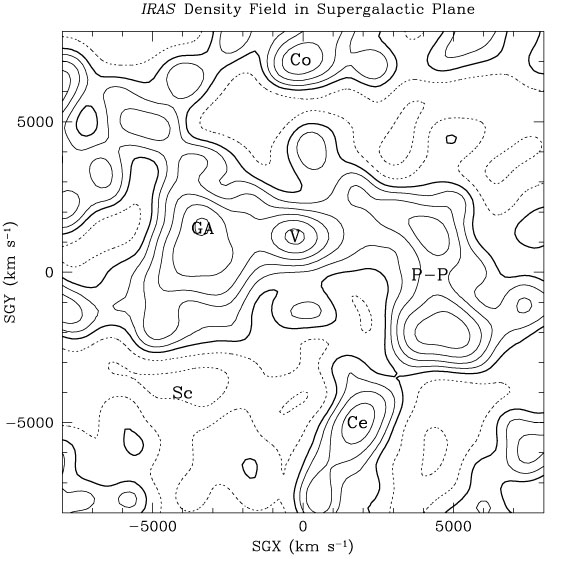
Figure 6. The density field of IRAS galaxies in the Supergalactic plane. A 500 km s- 1 Gaussian smoothing has been applied. Prominent structures are labeled: V = Virgo, GA = Great Attractor, P-P = Perseus-Pisces, Co = Coma-A1367 Supercluster, Sc = Sculptor Void, and Ce = Cetus Wall. |
The slice through the Supergalactic plane (Supergalactic Z = 0) is
shown in Fig. 6. The contours are of the
galaxy density field  (Eq. 24). The heavy contour is at the mean density,
= 0, while the dashed
contours are at
= - 1/3 and -2/3. The solid
contours
represent positive values of
and are logarithmically spaced
in 1 + , with three contours
corresponding to an increase of a
factor of two. One's first visual impression from these maps is the
irregularity of the shapes of the largest structures. One sees
immediately that modeling superclusters as uniform spheres can be
misleading! One also notes the rough symmetry between the high and
low-density regions. If the distribution function of the primordial
density field is symmetric between under-dense and overdense regions,
then linear theory predicts this symmetry to be preserved. However,
because is has a strict
lower limit of -1, while there is
no corresponding upper limit, we expect a positive skewness to develop
for late enough times and small enough smoothing scales that
< 2 >
approaches unity (Section 5.4). This is
evident
in the maps here, although there is still a rough balance between the
volume of space occupied by over- and under-dense regions. One can do
statistics with the topology of the isodensity contours; we
will discuss this in Section 5.6.
(Eq. 24). The heavy contour is at the mean density,
= 0, while the dashed
contours are at
= - 1/3 and -2/3. The solid
contours
represent positive values of
and are logarithmically spaced
in 1 + , with three contours
corresponding to an increase of a
factor of two. One's first visual impression from these maps is the
irregularity of the shapes of the largest structures. One sees
immediately that modeling superclusters as uniform spheres can be
misleading! One also notes the rough symmetry between the high and
low-density regions. If the distribution function of the primordial
density field is symmetric between under-dense and overdense regions,
then linear theory predicts this symmetry to be preserved. However,
because is has a strict
lower limit of -1, while there is
no corresponding upper limit, we expect a positive skewness to develop
for late enough times and small enough smoothing scales that
< 2 >
approaches unity (Section 5.4). This is
evident
in the maps here, although there is still a rough balance between the
volume of space occupied by over- and under-dense regions. One can do
statistics with the topology of the isodensity contours; we
will discuss this in Section 5.6.
In this figure, the Local Group sits at the origin. Some of the
prominent structures are labeled with identifying flags. The nearest
substantial overdensity is found at
X = - 250 km s-1, Y = 1150
km s-1;
this is the Virgo Cluster
(15)
(V), the nearest large cluster of galaxies. The Ursa Major
cluster, a somewhat more diffuse and spiral-rich cluster, is too close
to Virgo to be resolved as a separate structure with this
smoothing. The traditional definition of the Local Supercluster refers
to it as a flattened structure in the Supergalactic plane of extent
 2000 km
s-1, with the Virgo cluster at its center (indeed, one
often hears the Local Supercluster referred to as the Virgo
Supercluster), but as this figure shows, the Local Supercluster is far
from an isolated structure. In particular, at this smoothing, it joins
with the Great Attractor (GA), which is the large extended
structure centered at
Z = - 3400 km s-1, Y = 1500
km s-1. The Great
Attractor is often referred to as two separate superclusters, the
Hydra-Centaurus (positive supergalactic Y) and
Pavo-Indus-Telescopium (negative supergalactic Y) Superclusters,
although that division is somewhat artificial, being imposed by the
zone of avoidance. The IRAS survey clearly shows the two
superclusters to be contiguous (the effective smoothing length is
greater than the width of the excluded zone). The Great Attractor was
first named as such by
Dressler (1987b)
,
when peculiar velocity
surveys showed a convergence in the galaxy velocity field towards a
point corresponding to the Hydra-Centaurus supercluster
(Lilje, Yahil, &
Jones 1986
;
Lynden-Bell et
al. 1988)
as we discuss in Section 7.1.2 below.
Subsequent redshift surveys (cf.
Strauss & Davis
1988
;
Dressler 1988
;
1991)
mapped the full extent of the
overdensity of galaxies associated with the Great Attractor. See
Lynden-Bell, Lahav,
& Burstein (1989)
for a brief history of
definitions of the Great Attractor. In the context of redshift
surveys, we define the Great Attractor as the extended overdensity of
galaxies that dominates the left hand side of
Fig. 6.
2000 km
s-1, with the Virgo cluster at its center (indeed, one
often hears the Local Supercluster referred to as the Virgo
Supercluster), but as this figure shows, the Local Supercluster is far
from an isolated structure. In particular, at this smoothing, it joins
with the Great Attractor (GA), which is the large extended
structure centered at
Z = - 3400 km s-1, Y = 1500
km s-1. The Great
Attractor is often referred to as two separate superclusters, the
Hydra-Centaurus (positive supergalactic Y) and
Pavo-Indus-Telescopium (negative supergalactic Y) Superclusters,
although that division is somewhat artificial, being imposed by the
zone of avoidance. The IRAS survey clearly shows the two
superclusters to be contiguous (the effective smoothing length is
greater than the width of the excluded zone). The Great Attractor was
first named as such by
Dressler (1987b)
,
when peculiar velocity
surveys showed a convergence in the galaxy velocity field towards a
point corresponding to the Hydra-Centaurus supercluster
(Lilje, Yahil, &
Jones 1986
;
Lynden-Bell et
al. 1988)
as we discuss in Section 7.1.2 below.
Subsequent redshift surveys (cf.
Strauss & Davis
1988
;
Dressler 1988
;
1991)
mapped the full extent of the
overdensity of galaxies associated with the Great Attractor. See
Lynden-Bell, Lahav,
& Burstein (1989)
for a brief history of
definitions of the Great Attractor. In the context of redshift
surveys, we define the Great Attractor as the extended overdensity of
galaxies that dominates the left hand side of
Fig. 6.
On the opposite side of the sky, there is an extended chain of galaxies with two distinct density peaks, at X = 4300 km s-1, Y = 1300 km s-1, and X = 4750 km s-1, Y = - 2000 km s-1. This is the Perseus-Pisces Supercluster (P-P), the Northern part of which is sometimes referred to as the Camelopardalis Supercluster. These contour plots do not give justice to the remarkable tightness and coherence of the galaxy distribution here; Giovanelli et al. (1986) show that the structure lies nearly in the plane of the sky, and displays a remarkably filamentary structure, with rich clusters embedded in it. There is a void in the foreground of the Perseus-Pisces supercluster centered at X = 2000 km s-1, Y = - 1400 km s-1. There is also a void beyond the Virgo cluster, which stretches to the Coma-A1367 supercluster (Co), centered at X = 0, Y = 7100 km s-1. This supercluster is embedded in the Great Wall (Fig. 3), although the Great Wall itself lies beyond the boundaries of this figure for the most part. The void centered at X = - 4000 km s-1, Y = - 4000 km s-1 was discovered by da Costa et al. (1988) ; Dekel & Rees (1994) refer to it as the Sculptor Void (Sc). Finally, the radially directed structure centered at X = 1800 km s-1, Y = 5000 km s-1 is the Cetus Wall (Ce), discovered by the SSRS.
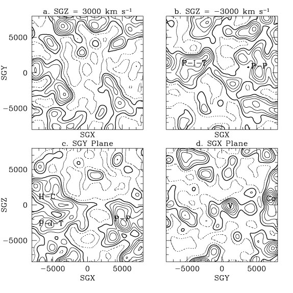
Fig. 7a is a slice at Z = 3000 km s-1, and shows that the region above the Supergalactic plane is marked by an extensive void. This void extends almost to the Local Group, and is apparent in the distribution of galaxies very near us as the Local Void (cf. Tully 1987b). The overdensity extending across the top of the figure is a piece of the Great Wall. Below the Supergalactic plane (Fig. 7b Z = - 3000 km s-1), one sees the extensions of the Great Attractor (in the form of the Pavo-Indus-Telescopium supercluster, P-I-T) and the Pisces-Perseus Superclusters.
|
Figure 7. The density field in various slices in Supergalactic coordinates a: Z = + 3000 km s-1. b: Z = - 3000 km s-1. c: Y = 0. d: X = 0. Prominent structures marked include H-C=Hydra-Centaurus, and P-I-T=Pavo-Indus-Telescopium. |
Panel c of Fig. 7 is the Y = 0 slice. This slice lies almost in the Galactic plane, and cuts cleanly through the Great Attractor (negative X) and the Northern part of the Pisces-Perseus Supercluster (positive X). The Great Attractor is seen to be bimodal in this cut, and we label the Hydra-Centaurus (H-C) and P-I-T superclusters separately. The extent of the void above the Supergalactic plane (Fig. 7a) is now clear; it occupies the entire upper part of this figure. A slice at X = 0 (Fig. 7d) passes through the Virgo cluster, and the Coma-A1367 superclusters. The Great Wall is apparent at Y = 7000 km s-1 in this slice.
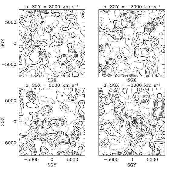
The slice at Y = 3000 km s-1 (Fig. 8a) shows no dramatic structures, and is largely dominated by the void that lies between the Local and Coma-A1367 superclusters. The slice at Y = - 3000 km s-1 (Fig. 8b) cuts through the southern (i.e., smaller Y) part of the Pisces-Perseus supercluster, and shows it to be extended in the Supergalactic Z direction. The region south of the Great Attractor is dominated by the Sculptor Void (Sc).
|
Figure 8. The density field in various slices in Supergalactic coordinates a: Y = + 3000 km s-1. b: Y = - 3000 km s-1. a: X = + 3000 km s-1. b: X = - 3000 km s-1. |
X = 3000 km s-1 (Fig. 8c) slices through the Pisces-Perseus supercluster, showing it to be multi-modal. Indeed, there is a void between the Perseus-Pisces Supercluster in the Supergalactic plane, and its counterpart at Z = - 3000 (Fig. 8b). Finally, the slice at X = - 3000 (Fig. 8d) cuts through the Great Attractor. The bimodality apparent in the Y = 0 slice is apparent here as well. The Sculptor Void appears here, bracketed by a remarkable wall of galaxies extending from the Great Attractor to the upper left hand corner of the figure.
In this brief overview of the galaxy distribution as seen by IRAS, we have not been comprehensive: we have not endeavored to give every structure that is visible a name, nor have we given justice to the detailed mapping that has been done by a large number of people (see the references above). Moreover, with our 500 km s- 1 Gaussian smoothing, we have washed out some of the more remarkable structures that are apparent in the redshift data: the very thin walls and filaments, and the tight clusters. However, the main emphasis in this survey is on quantitative and statistical analyses of the galaxy distribution, and thus we now move beyond cosmography, to see what quantitative science we can do with the data presented here.
15 It is standard practice to name clusters and superclusters after the constellations in which they are found. Back.