7. STATISTICAL MEASURES OF THE VELOCITY FIELD

We begin this chapter with a discussion of bulk flows in Section 7.1; this has been the major theme of much of the work in peculiar velocities in the last decade. Section 7.2 summarizes the history of peculiar velocity work with a discussion of the effort needed to put on a common basis the various samples available. The rest of the chapter discusses various statistics measurable from the observed flow field. The velocity correlation function and the Cosmic Mach Number are discussed in Section 7.3 and Section 7.4, respectively. Section 7.5 is devoted to derivations of the full three-dimensional velocity field from its radial component, with emphasis on the POTENT technique of Bertschinger & Dekel (1989) , and the results that have come from this work.

7.1. A History of Observations of Large-Scale Flow

Since the mid-1970's coherent departures from uniform Hubble flow ⁽³¹⁾ have been observed on ever larger scales. A comprehensive historical review of the subject through ~ 1989 is given by Burstein (1990) . Here we briefly outline this history from ~ 1976 to the present, with an emphasis on recent years.

When one speaks of a coherent bulk flow, one requires a velocity frame of reference. Prior to the mid-1970's, the most logical choice for such a frame was that defined by the barycenter of the Local Group of galaxies (LG), the bulk of whose mass is found in the Milky Way and the Andromeda galaxy M31. Our own motion with respect to such a frame was thought to arise from LG dynamics and the rotation of the Milky Way; the LG barycenter itself was considered at rest with respect to the Hubble expansion. This reasoning changed following the discovery of the CMB dipole anisotropy in 1976 (see Section 5.7). The CMB dipole was and is most naturally interpreted as due to the motion of the LG with respect to the rest frame of the totality of mass within our observable universe, in the direction l = 276°, b = 30°, and with amplitude 627 km s^-1. With this finding it became clear that significant peculiar velocities exist in the Universe: unless the LG is atypical, peculiar motions of hundreds of km s^-1 could no longer be considered unusual. The CMB dipole also suggested a natural reference frame for the analysis of peculiar motions.

7.1.1. Early Work

The first claimed detection of large-scale streaming was that of Rubin et al. (1976a, b), who assumed that giant Sc spiral galaxies are standard candles. They studied a sample of 96 such galaxies in the redshift range 3500-6500 km s^-1, and found a bulk flow relative to the Local Group frame of ~ 600 km s^-1 in the direction l = 160°, b = - 10°. The Rubin et al. result provoked a great deal of skepticism in the astronomical community, despite the (nearly simultaneous) discovery of the CMB dipole. The direction of the Rubin et al. bulk flow was nearly orthogonal to the LG velocity vector, making the relationship of the two measurements difficult to understand. Indeed, the measurement of Rubin et al. to this day has neither been confirmed nor entirely refuted, but instead has simply been supplanted by more modern data based on better distance indicators.

In the late 1970s and early 1980s, peculiar velocity work focused on the detection of infall to the Virgo cluster, which lies near the North Galactic Pole at 270°, b 75°, and is the nearest large cluster to the Local Group. A number of workers using TF, Faber-Jackson, and other techniques estimated the amplitude of this motion at the Local Group to be in the range ~ 150-400 km s^-1 (e.g., Schechter 1980 ; Aaronson et al. 1982a; de Vaucouleurs & Peters 1981 ; Tonry & Davis 1981a , b; Hart & Davies 1982 ; Dressler 1984). Even if the largest of these estimates were correct, the misalignment between the Virgo direction and the CMB dipole meant that Virgocentric infall could not be the sole cause of the LG motion (Davis & Peebles 1983a ; de Vaucouleurs & Peters 1984 ; Sandage & Tammann 1984 ; Yahil 1985). This led to suggestions that the remaining part of the LG motion resulted from the pull of the relatively nearby Hydra-Centaurus supercluster complex, which lies almost near the apex of the microwave dipole at a redshift cz 3000 km s^-1 (Shaya 1984 ; Tammann & Sandage 1985 ; Davies & Stavely-Smith 1985). Lilje, Yahil, & Jones (1986) studied residuals from the Virgocentric flow solution of Aaronson et al. (1982a) and concluded they were best fit by a quadrupolar term arising from the pull of Hydra-Centaurus. These suggestions were consistent with the generally accepted view that peculiar motions arose from relatively "local" (scales 5000 km s^-1) mass density perturbations.

7.1.2. 1986-1990: The "Great Attractor"

Confirmation of this view appeared to come from a long term study by the Aaronson group. Using IRTF distances to ten clusters in the 4000-10,000 km s^-1 redshift range, Aaronson et al. (1986) concluded that these clusters exhibited no net motion relative to the CMB ⁽³²⁾ . They argued, as a corollary, that the LG motion had to be entirely generated by mass fluctuations within ~ 5000 km s^-1. The picture that prevailed in the mid-1980's was thus one in which the Hubble flow was unperturbed on scales 5000 km s^-1. But within several years the paradigm had changed radically, due mainly to the work of the "7 Samurai" (7S). Applying the D_n- relation to an all-sky sample of over 400 bright (m_B 13 mag, <cz> 3000 km s^-1) elliptical galaxies, the group reported a bulk flow of amplitude 600 ± 100 km s^-1 relative to the CMB frame, in the direction l = 312 ± 11°, b = 6 ± 10° (Dressler et al. 1987a). They emphasized that galaxies in the Hydra-Centaurus concentration participated in, and therefore could not be the source of, the observed flow. They concluded that, contrary to the conventional wisdom, the greater part of the LG motion relative to the CMB had to be generated on scales 5000 km s^-1.

This result shook up the cosmology community considerably. Its significance lay not so much in the amplitude as in the coherence scale of the flow. Indeed, as initially reported by Dressler et al. (1987a) , the true scale of the bulk flow was unconstrained, potentially larger than the effective limit (~ 6000 km s^-1) of their sample. It was quickly realized (e.g., Vittorio, Juszkiewicz, & Davis 1986) that a bulk flow on this scale was inconsistent with essentially all of the then-popular scenarios for large-scale structure formation, including the standard cold and hot dark matter models. The power spectrum P(k) for any of those models did not contain sufficient power on large scales to generate flows of amplitude ~ 600 km s^-1 on scales 5000 km s^-1 (Eq. 40). Kaiser (1988) showed that the situation for cosmological models was not as dire as Vittorio et al. (1986) implied, as the effective depth of the 7S sample was not as large as had been assumed. Indeed, the fitted bulk flow was not inconsistent with the standard CDM model with high enough normalization. However, in this case, the small-scale velocity dispersion is larger than that observed; Bertschinger & Juszkiewicz (1988) point out that there is no normalization of standard CDM which can simultaneously match the 7S bulk flow and the observed small velocity dispersion (cf., Section 7.4).

The controversial nature of the 7S result was at least partially alleviated when the group undertook a reinterpretation of their data in Lynden-Bell et al. (1988a, hereafter LB88). They showed that much of the signal for the elliptical streaming motion was provided by galaxies within ~ 2000 km s^-1; if they confined their analysis to objects at distances 3000 km s^-1, bulk flow was only marginally detected. Moreover, in a conical region within ~ 60° of the apex of the apparent bulk flow, the derived amplitude was nearly 1000 km s^-1. They interpreted this as due to infall into an attracting point. They fit their data using a Method I approach (Section 6.4) to a model in which the flow is generated primarily by a spherically symmetric density perturbation they called the "Great Attractor" (GA) (cf., Section 4). In addition to the GA distance and flow amplitude, which were treated as free parameters, the model of LB88 included a Virgo infall motion with a fixed amplitude of 250 km s^-1 at the position of the LG. Their maximum-likelihood fits placed the GA at a distance of 4350 ± 350 km s^-1 in the direction l = 307°, b = 9°, indicated that it induced an infall velocity of 570 ± 60 km s^-1 at the position of the LG, and attributed to it a mass of ~ 5.4 × 10¹⁶ M.

A further elaboration of the GA model was provided by Faber & Burstein (1988, FB88), who combined TF data for nearby spirals from Aaronson et al. (1982b) with the 7S elliptical data. FB88 fitted the combined data set to a model in which the local velocity field was fully described by infall motions into the GA and Virgo, but with the parameters characterizing each motion allowed to vary independently (see also Han & Mould 1990). They obtained consistent results using Method I and Method II analyses. Two important conclusions resulted from this work. First, the nearby TF spirals (cz 2500 km s^-1) mapped out a velocity field similar to that of the ellipticals. Second, the effect of Virgo was found to be very small in comparison with the tidal effect of the GA: the infall motion due to Virgo alone at the position of the LG had an amplitude of ~ 100 km s^-1. This contrasted strongly with earlier estimates (e.g., Aaronson et al. 1982a) which had found a Virgocentric motion of ~ 300 km s^-1 and higher (Section 7.1, Section 8.1.1). FB88 verified that the discrepancy between their Virgo flow solution and that of Aaronson et al. was due solely to the shear caused by the GA in the model (cf., Lilje et al. 1986) ⁽³³⁾ .

Apparent confirmation of the GA picture came from two directions. First, three newly-completed redshift surveys (da Costa et al. 1988 ; Dressler 1988 ; Strauss & Davis 1988) showed that there was in fact a very strong excess number of galaxies in the direction of the proposed GA, peaking at cz ~ 4000 km s^-1 (cf., Fig. 6). The second source of support for the GA model came from further peculiar velocity studies of the region. Aaronson et al. (1989) extended their infrared TF cluster study to the Hydra, Centaurus, and other neighboring clusters and confirmed large positive peculiar velocities for these clusters (see also Mould et al. 1991). Dressler & Faber (1990a, b) studied field galaxies in the GA region using both the TF (using CCD photometry and optical linewidths) and D_n- methods. Probing deeper than earlier studies, they claimed to detect "back-side infall" into the GA, i.e., negative peculiar motions of galaxies at distances 5000 km s^-1. Such motions would have to exist if the positive velocities detected in the foreground were indeed generated by the GA, and the GA was an isolated structure. The detection of backside infall remains controversial (cf., Burstein et al. 1990; Roth 1993 ; Mathewson & Ford 1994), given the large and uncertain correction for inhomogeneous Malmquist bias. In addition, it is clear that the velocity field within the Centaurus cluster is quite complex; it consists of two pieces with substantially different distances and peculiar velocities (e.g., Lucey, Currie, & Dickens 1986; Burstein et al. 1990).

7.1.3. 1990-1994: Very Large-Scale Streaming?

Several independent peculiar velocity surveys came to fruition around 1990, with results that challenged the consensus which had emerged around the GA picture. Willick (1990, 1991; hereafter W91) reported an R band CCD TF study of 155 cluster spirals from the sample of Aaronson et al. (1986) , and of 326 field spirals in the Perseus-Pisces supercluster region (PP). One of the more prominent structures in the nearby universe (Fig. 6), PP consists of a dense filament of galaxies at redshift ~ 5000 km s^-1, centered on l ~ 110°, b ~ - 30°. W91 obtained velocity widths for PP galaxies from the published 21 cm data of Giovanelli & Haynes (1985, 1989) and Giovanelli et al. (1986). The W91 PP sample was concentrated in a relatively narrow (~ 15°) strip in galactic latitude, stretching over ~ 90° in longitude. PP lies nearly opposite on the sky from the GA at a similar distance, but was not well sampled in the 7S study. The PP region thus represented a significant uncharted volume in the velocity field as mapped by the elliptical data.

W91 used the cluster galaxies to calibrate the R band TF relation, assuming (following the finding of the Aaronson group) that the Northern Sky clusters were at rest in the CMB. When applied to the PP galaxies, the TF data revealed a coherent motion directed toward the LG, with a mean amplitude of ~ 350 km s^-1. Superposed on the coherent streaming were compressional motions presumably due to the overdense PP filament, but the bulk motion was the most prominent feature of the data. Because of the location of PP, the streaming motion was directed not only toward the LG, but also approximately toward the GA. The amplitude of this streaming was much larger than what was predicted at PP (~ 150 km s^-1) by the FB88 GA model. W91 suggested that the residual motion might be due to very large-scale, low amplitude density fluctuations, but noted that at the largest distances in his sample (~ 10,000 km s^-1), objects appeared to be at rest in the CMB frame.

The small solid angle covered by the W91 PP sample raised the question of whether the PP inflow extended over a larger region of the sky. Confirmation that it did was provided by the R band CCD TF survey of Courteau and Faber (Courteau 1992 ; Courteau et al. 1993 ; CF), who obtained data for 321 galaxies distributed over the Northern sky using a dilute sampling approach. CF used optical H rotation curves to measure velocity widths. Because of their large sky coverage and very uniform selection criteria, CF were able to compare different regions of the sky reliably. Well away from PP their data suggested a relatively quiescent velocity field, as indicated by the small scatter of the TF relation when distances were modeled by pure Hubble flow. However, within the PP region - now defined to cover an area several times larger than the W91 sample - the scatter was larger and the residuals systematically offset from Hubble flow. The implied velocity was ~ 300-350 km s^-1 toward the LG, in agreement with W91. Further confirmation of a bulk motion came from Han & Mould (1992) , who used the I band CCD TF relation to study five clusters embedded in the PP supercluster. They found PP to be moving towards the LG with amplitude ~ 400 km s^-1.

Han, Mould and collaborators also obtained I band TF data for 16 further clusters distributed over much of the sky (Han 1992 ; Mould et al. 1991). This sample of clusters largely overlapped those studied using the IRTF by Aaronson et al. (1986, 1989), but the I band relation was considered more accurate. Han & Mould (1992) fitted the combined data for 21 clusters to two models: a large-scale bulk streaming similar to the original model proposed by the 7S group (Dressler et al. 1987a); and a "bi-infall" model in which the local universe is dominated by competing gravitational pulls of the GA and Perseus-Pisces. They found that both models were consistent with the data.

Connolly (1993) measured Tully-Fisher parameters for a sample of 218 Sc galaxies in both Galactic hemispheres, with mean redshift of 5500 km s^-1. He fits the data to a dipole and finds good agreement with the analysis of a much larger sample by Courteau et al. (1993) .

The largest single contribution of Tully-Fisher data in recent years has been that of Mathewson and collaborators (Mathewson et al. 1992a, b, hereafter MAT92; Mathewson & Ford 1994). Using I band CCD photometry and a combination of HI and optical velocity widths from several telescopes in Australia, MAT92 obtained TF data for 1355 Southern sky galaxies. Roughly half of these were in the steradian around the GA region as defined by the 7S group, and another half, thought of as a control group, were outside. The sample was constructed to be roughly complete to an ESO diameter limit of 1.7'. Most objects in the sample have redshifts 4000 km s^-1, but a substantial number have 5000 cz 7000 km s^-1. MAT92 calibrated their TF relation relative to ~ 40 galaxies with TF data from Aaronson et al. (1989) , Willick (1991) , and Han & Mould (1992) .

The redshift vs. TF distance diagram for galaxies in the "control" region exhibited pure Hubble flow in the mean. Within the GA region, MAT92 confirmed the large (~ 1000 km s^-1) outflowing motions in the GA foreground that had been detected in the 7S elliptical data. However, the spirals did not appear to trace a velocity field which fell to zero at the distance (~ 4500 km s^-1) of the nominal Great Attractor. Instead, the data indicated that the GA itself (i.e., galaxies in the redshift range ~ 4000-5000 km s^-1) possessed a mean positive peculiar velocity of ~ 600 km s^-1. Furthermore, the MAT92 data did not exhibit the "backside infall" which Dressler & Faber (1990ab) had claimed to detect: even at distances 000 km s^-1 a return to the Hubble line was not apparent. MAT92 argued that their data, in combination with those of Willick (1990) , suggested a vast bulk flow in the Supergalactic plane on scales well in excess of 10,000 km s^-1.

However, a recent reanalysis of the MAT92 data, as well as further data from the Mathewson group itself, have not lent support to this hypothesis. MAT92 did not attempt a careful correction for selection or Malmquist biases; in addition, their zeropoint calibration used only a small number of independent comparisons. Using a careful zeropointing technique which ties together the distance scale of several TF samples, Willick et al. (1995a, b, c) have recalibrated the TF relations used by MAT92 as well as other TF samples (see Section 7.2). Preliminary analyses of the recalibrated data (Courteau et al. 1993 ; Faber et al. 1993 , 1994) have derived modest (~ 300-350 km s^-1) bulk flows in the GA direction, as well as evidence of a return to the Hubble line at the distance of the GA. The backside infall, however, remains undetected in these recent studies. Very recently, Mathewson & Ford (1994) have enlarged their Southern sky sample by ~ 1000 galaxies. The new sample is selected to an ESO diameter of 1' and thus probes to greater distances (cz 10, 000 km s^-1). Mathewson & Ford measure a bulk flow in the GA direction of ~ 370 km s^-1 for the combined sample, in good agreement with Courteau et al. (1993) , and a return to the Hubble line at cz 7000 km s^-1. The new data have not been reanalyzed using the techniques of Willick et al.; this will be carried out in the near future.

7.1.4. The Lauer-Postman Result

The most dramatic apparent detection of very large-scale streaming to date comes from the work of Lauer & Postman (1994, hereafter LP). Using the BCG L- relation (Section 6.3.2), LP obtained redshift-independent distances to a volume-limited sample of 119 Abell clusters in the redshift range cz < 15, 000 km s^-1. The typical distance error from the method was estimated by LP as ~ 16%, so that the peculiar velocity error for a typical sample cluster is ~ 2000 km s^-1, much too large to estimate individual cluster peculiar velocities. However, the data do allow the determination of a mean bulk velocity vector for the sample.

LP defined an "Abell Cluster Inertial Frame," or ACIF, and measured the velocity of the LG L relative to it. They solved for L by minimizing the ²-like quantity ⁽³⁴⁾

(200)

where:

1. _i is the -value for galaxy i;
2. z_i its redshift in the LG frame;
3. M(_i) is its residual (in magnitudes) from the L- relation;
4. _i is a unit vector toward the galaxy; and
5. L is the motion of the LG with respect to the ACIF.

The minimization is carried out with respect to the parameters specifying the L- relation (which determine the quantity M()), and the three components of L. The quantity (2 - ) which appears both in the weighting term and in the exponent arises from the fact that both L and must be measured within metric apertures; as a result the effective scatter of the relation is actually given by 2_M / (2 - ) where _M = 0.24 mag is the scatter about the relation. The z^-2 term gives greatest weight to the nearby clusters, although LP show the solution is insensitive to the redshift weighting.

LP found that the LG motion relative to the ACIF was in the direction l = 220°, b = - 28° (total angular uncertainty ± 27°). That the LG would have a significant motion relative to an inertial rest frame is of course no surprise; we already know that the LG moves at ~ 600 km s^-1 relative to the CMB. However, the latter motion is in the direction l = 276°, b = 30° (with negligible angular uncertainty). Consequently, according to LP the ACIF differs significantly from the frame defined by the CMB dipole. Stated another way, if the CMB defines the true cosmic rest frame, the LP data indicate that the Abell clusters out to 15,000 km s^-1 possess a net peculiar motion of 689 ± 178 km s^-1 in the direction l = 343°, b = + 52 (total angular uncertainty ± 23°). Aware of the controversial nature of their result, LP performed a suite of tests aimed at identifying systematic effects in their analysis. Among other things, they considered the effects of cutting their sample at low and high redshifts, and at low and high values of , of removing prominent superclusters (such as the Hydra-Centaurus complex) from their sample, of using a linear rather than a quadratic L- relation, and of removing galaxies with very large residuals. They found that none of these tests produced significant changes in their solution. They did identify one non-negligible systematic effect called "geometry bias," which arises due to coupling between the dipole moment of the sky distribution of the sample and the distance indicator relation. LP calibrated and corrected for this effect using Monte Carlo experiments; in practice, it was rather small (< 100 km s^-1) since their sample has excellent sky coverage.

One could take the view that a ~ 700 km s^-1 bulk motion of a volume ~ 30,000 km s^-1 in diameter is highly implausible, and attribute it instead to an incorrect choice of cosmic rest frame. One would then be obliged to jettison the conventional view that the CMB dipole is kinematic in origin; possible explanations of a cosmological origin for the CMB dipole have been suggested by Gunn (1988) , Paczynski & Piran (1990) , and Turner (1991) . While the possibility that the CMB does not define a cosmic rest frame cannot be excluded, such a view has become increasingly difficult to uphold in light of the discovery of small but measurable CMB anisotropies by the COBE satellite (Smoot et al. 1992). These COBE measurements have corroborated most theoretical ideas about the nature of the CMB.

Alternatively, if one accepts the kinematic origin of the CMB dipole and the resultant CMB-defined rest frame, the LP data indicate a ~ 5% perturbation to the Hubble flow on a 15,000 km s^-1 scale. This is difficult to reconcile with bulk flow observations from the TF and D_n- relations. Courteau et al. (1993) used the Mark III dataset (Section 7.2) to estimate the bulk flow within 6000 km s^-1 to have an amplitude of 360 ± 40 km s^-1 in a nearly orthogonal direction, toward 300°, b + 10°. It is difficult to understand how the amplitude of the bulk flow could grow with scale in a universe which approaches uniformity in the galaxy distribution in the large, especially given the apparent convergence of the dipole in the galaxy distribution between 6000 and 15,000 km s^-1 (Section 5.7).

The LP result also poses severe problems for a number of currently popular theories for the growth of large-scale structure. Strauss et al. (1995) have generated mock LP-like BCG samples in N-body simulations based on six different cosmogonic scenarios, including CDM, HDM, and PIB models. These mock samples were constructed to mimic all the observational errors in the actual LP sample. Strauss et al. found that no more than 2-5% of the realizations of any given model exhibited an apparent flow as large as that measured by LP. Similar results were found by Feldman & Watkins (1994) using an analytic approach. Jaffe & Kaiser (1995) suggest comparing not just the bulk flow, but the full sample of peculiar velocities, to the predictions of various models. They find better agreement between the LP data and models than do Strauss et al. and Feldman & Watkins. However, as Jaffe & Kaiser ignore the correlations between the measured peculiar velocities of different clusters, which arise from the self-calibrating nature of the LP sample, the validity of their analysis is uncertain.

The very careful treatment by LP makes it unlikely that the observed flow will "go away" with a future reanalysis of the data. Rather, it seems likely that future measurements on comparably large scales (Section 9.7) will determine the ultimate evaluation of LP, as was the case with the Rubin et al. (1976a, b) result. If LP is confirmed, it will need to be reconciled with the discrepant flows seen on smaller scales, and theoretical models are likely to require significant revision.

7.1.5. Bulk Flows: A Summary

The myriad of bulk flow analyses we have discussed here have used a wide variety of samples, methodologies and techniques, and have been carried out during a time when our knowledge of the properties of distance indicators, and the various biases which plague them, was evolving rapidly (as indeed it still is). The bulk flows measured by different samples necessarily probe different volumes of space; a direct comparison between them is problematic, and we have not attempted one in this review. Nevertheless, there is a rough consensus between the different workers in the field as to the nature of the bulk flow within 6000 km s^-1 (cf., the review by Postman 1995), both in its amplitude and in its direction. Even the Lauer-Postman bulk flow, which is on appreciably larger scales than the others, agrees very roughly in direction. The surprising thing about this result is the fact that it also agrees roughly in amplitude, on such a large scale.

One of our aims in measuring bulk flows is to compare with theoretical predictions, as given for a given model by Eq. (40). This equation refers to the volume-weighted average of the three-dimensional velocity of particles within a spherical volume, which can differ substantially from the galaxy- and error-weighted average of radial velocities that is usually measured. Indeed, as Juszkiewicz et al. (1990) and Strauss et al. (1995) point out, one can have a bulk flow within a volume even in the absence of density fluctuations on larger scales, if the center of mass of the volume does not coincide with its geometric center. There are a number of such subtleties which are only now being appreciated in this game; further theoretical analyses along the lines of Kaiser (1988; 1991) and Feldman & Watkins (1994) are needed.

Of the samples discussed here, only that of Lauer & Postman (1994) approached being volume-limited (cf., Roth 1993 , 1994). However, one can measure an effective volume-limited bulk flow if one weights the galaxies appropriately. The POTENT technique (to be discussed in detail in Section 7.5) does exactly that, and Bertschinger et al. (1990) quote volume-limited bulk flows measured within a series of spheres centered on the Local Group. More recent results using POTENT applied to a more complete data set by Dekel et al. (1995) show a bulk flow of 400 km s^-1 within a sphere of radius 6000 km s^-1, which is in fact consistent with standard CDM normalized to COBE. Again, the Lauer-Postman result, which probes appreciably larger scales, is in disagreement with this and all other viable models; we suspect that measurements of bulk flows on large scales will continue to be a very active area of research for at least the next five years.

7.2. Homogeneous Peculiar Velocity Catalogs

Tully-Fisher and D_n- data have been collected, at an increasing rate, over the past fifteen years. There now exists a large number of independent data sets potentially useful in peculiar velocity surveys. This trend will accelerate in the coming years, as most ordinary spiral and elliptical galaxies out to ~ 10,000 km s^-1 acquire quality photometric and spectroscopic measurements. There is and will be a need for uniform catalogs containing the TF and D_n- observable data, and the corresponding estimated distances and peculiar velocities. Distances obtained using the newer DIs such as the PNLF, SBF, BCG, and SNe methods will eventually be cataloged as well.

The greatest problem in constructing a peculiar velocity catalog is ensuring the homogeneity of the separate samples. The originally published inferred distances to galaxies found in two or more independent data sets are almost sure to differ systematically, for two basic reasons. First, observers measure the relevant quantities - apparent magnitudes, diameters, and internal velocity widths - differently; they not only use different observational methods, but apply different corrections (e.g. for internal extinction) to the raw observables. As a result, there are as many TF relations (say) as there are data acquisition and reduction techniques. Nonetheless, a TF relation derived for one data set is sometimes heedlessly applied to another. Second, observers determine the appropriate TF relation (say) from their data in different ways. Some fit an inverse relation, some a forward relation; in each case, the treatment (if any) of selection bias can differ. A naïvely constructed peculiar velocity catalog, in which inferred distances are simply appropriated from the published literature, will thus be plagued with systematic errors within and between data sets.

Until recently, attempts to produce uniform peculiar velocity catalogs from the literature have been largely the work of D. Burstein, a member of the 7S collaboration. Two early versions known as the Mark I and Mark II, were distributed privately to the community by electronic mail in 1987 and 1989 respectively. Burstein tabulated the D_n- elliptical galaxy data of the 7S group, Lucey & Carter (1988) and Dressler & Faber (1990a) , as well as the infrared TF spiral data of the Aaronson group. Burstein was able to make direct comparisons of the D_n- data from the different groups. However, it was difficult to guarantee that the spiral and elliptical data were on the same system; comparison of TF and D_n- group distances was used to make small adjustments, but these comparisons suffered from the inevitable uncertainty associated with the spatial segregation of spiral and elliptical galaxies. Although not optimal, the Mark II catalog played an important role in some of the major statistical studies of peculiar velocity in recent years (e.g., Bertschinger et al. 1990 ; Dekel et al. 1993).

With the advent of new large samples of peculiar velocity data, there has been a strong need to extend Burstein's effort, particularly in view of the more complete understanding of bias effects acquired in recent years (Section 6.5). A group led by one of the present authors (J.W.) has recently completed this task. The basic methodology is described in Willick et al. (1995a, b); the Mark III Catalog of Galaxy Peculiar Velocities is presented in Willick et al. 1995c, and is available for electronic distribution as well. The Mark III consists of the CCD TF samples of Han, Mould, and collaborators (Han 1991 , 1992; Han & Mould 1992 ; Mould et al. 1991, 1993; collectively, HM); Willick (1991, W91); Courteau and Faber (Courteau 1992 ; CF); and Mathewson et al. 1992b; and of the infrared TF sample of Aaronson et al. (1982b) , as recently reanalyzed by Tormen & Burstein (1994, 1995), who corrected previously unrecognized systematic errors in the diameter system used by the Aaronson group (see Section 6.1.1). The Mark III catalog will also include expanded versions of the elliptical D_n- samples found in the Mark II.

Several basic principles guide the construction of the Mark III catalog. The first is the adoption of a uniform set of rules for correcting the raw observable quantities, in particular apparent magnitude and velocity width, for the effects of extinction, inclination, and redshift. Internal extinction corrections have been a source of particular controversy in the past (see Burstein et al. 1995 for a review); the Mark III compilation adopts bandpass-specific internal extinctions which minimize TF scatter. The second principle is to re-derive a Tully-Fisher relation for each sample separately, taking full account of and correcting for selection biases in the manner suggested by Willick (1994; cf. Section 6.5). An important result of this re-derivation is that the TF relations in the Mark III compilation can differ markedly from those of the original authors. Third, the zeropoints (the constant A in Eq. 152) of the individual TF relations are mutually adjusted to yield the maximum agreement in the inferred distances for several hundred galaxies which are common to two or more individual samples. Finally, the global catalog zeropoint is determined by assuming that in the sample as a whole, the volume-weighted radial peculiar velocity component vanishes in the mean.

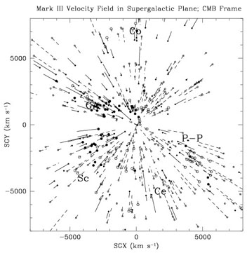
A representation of the Mark III velocity field is shown in Fig. 16, which shows the measured radial peculiar velocities of all galaxies within 22.5° of the Supergalactic plane. The point is drawn at the measured distance of the galaxy, while the line is drawn to its redshift, in the CMB rest frame. Positive peculiar velocities are drawn with solid points and solid lines, while negative peculiar velocities use open points and dashed lines. When possible, galaxies are grouped in order to decrease the errors and reduce the Malmquist bias; points representing groups of more than three galaxies are drawn somewhat larger. The zone of avoidance is apparent as the missing wedge out of the middle of the figure. Compare this figure with the IRAS density field of Fig. 6; we have labeled the major structures as we did in that figure. The bulk flow into the GA is apparent, as is the coherence of the flow even back to the Pisces-Perseus supercluster. It is difficult, however, to draw quantitative conclusions from this figure alone about bulk flows or infalls into specific structures. In the remainder of this chapter, we discuss various statistical analyses of peculiar velocity data, culminating in reconstruction methods of the full three-dimensional velocity field in Section 7.5.

Figure 16. The Mark III peculiar velocities of all galaxies within 22.5° of the Supergalactic plane. The point is drawn at the measured distance of the galaxy, while the line is drawn to its redshift, in the CMB rest frame. Positive peculiar velocities are drawn with solid points and solid lines, while negative peculiar velocities use open points and dashed lines. Points representing groups of more than three galaxies are drawn somewhat larger.

7.3. Velocity Correlation Function

One of the most striking features of the observed large-scale velocity field is its coherence. One way to quantify this is by fitting bulk flows to the data (Section 7.1). Another approach was suggested by Górski (1988) : the correlation function of the velocity field. Górski defines the correlation function between the ith and jth Cartesian component of the velocity field as:

(201)

where and _|| are the transverse and radial correlation functions. The second equality holds if the velocity field is homogeneous and isotropic. If the velocity field is derivable from a potential, then these two are not independent:

(202)

In linear perturbation theory, one can derive simple expressions for these quantities:

(203)

and

(204)

compare with Eq. (40). Of course, we observe only the radial component of the velocity field. Górski et al. (1989) and Groth, Juszkiewicz, & Ostriker (1989) have suggested methods to determine the velocity correlation function from observational data. The first of these papers defines a quantity from a sample with radial peculiar velocities u_i:

(205)

where the sum is over all pairs of galaxies with separations between r and r + r, and ₁₂ is the angle between galaxies 1 and 2 on the sky. A uniformly selected full-sky sample exhibiting a bulk flow of amplitude v will have a velocity correlation function ₁ = v² / 3. The second equality of Eq. (201) implies that (r) is a linear combination of _||(r) and (r), with coefficients depending on the spatial distribution of galaxies in the sample.

The velocity correlation function at zero lag is a measure of the root-mean-square velocity dispersion of galaxies, while the scale on which it drops to zero is a measure of the coherence length of the velocity field. Górski et al. (1989) looked at two datasets: the spiral galaxies of Aaronson et al. (1982) and the elliptical galaxies of the 7 Samurai. The correlation function of both drop to zero at separations of 2000 km s^-1. The amplitude of the elliptical galaxy dataset has a much larger amplitude than that of the spirals, although this amplitude was not robust: deleting a small number of galaxies in the Great Attractor region caused the amplitude to drop by more than a factor of two. These results were compared to N-body simulations of CDM and PBI models. The CDM models fit the observed correlation length well, and required a normalization ₈ > 0.5 to match the amplitude. The PBI models tended to show more coherence than is seen in the real data.

Groth et al. (1989) used the linear relation between and , _|| to solve for the latter. They emphasized the fact that in the frame comoving with the bulk flow of the Aaronson et al. (1982) data, the velocity correlations were essentially zero; the flow was very cold. This is consistent with the small value of the pairwise velocity dispersion deduced from redshift surveys (Section 5.2.1). Seen in this light, the correlation length of 2000 km s^-1 reported by Górski et al. (1989) is probably at least partly an edge effect due to a finite sample. It is time to revisit the velocity correlation function now that the data samples have improved and expanded. More work is needed to characterize the effects of survey geometry, and in particular, peculiar velocity errors, on this statistic. It has the potential to place strong constraints on cosmological models, once these various effects are understood better.

Juszkiewicz & Yahil (1989) point out that the comparison of the velocity and the spatial correlation function yields an estimate of ; in particular, in linear theory:

(206)

Note that the velocity correlations in this form on scale r depend only on the correlation functions on scales smaller than r. Thus accurate measurements of the velocity correlation function and the spatial correlation function have the potential to yield a measurement of . Moreover, the extent to which the two sides of Eq. (206) agree with one another as a function of r on linear scales is a test of gravitational instability theory. Unfortunately, existing data are not yet at the stage to allow this test to be done.

7.4. The Cosmic Mach Number

Ostriker & Suto (1990), struck by the coldness of the velocity field observed in the Aaronson et al. (1982) data, suggested a new statistic to quantify this coldness: the Cosmic Mach Number. The Mach number in standard usage is the ratio of the flow velocity in some medium to the sound velocity in that medium. In the cosmological context, the equivalent of the sound velocity is the small-scale velocity dispersion of galaxies. Following Eq. (40), the characteristic bulk velocities in a given cosmological model measure the large-scale component of the power spectrum, while the small-scale velocity dispersion depends on the power on small scales. Their ratio is thus independent of the amplitude of the power spectrum (at least in linear theory), and is a diagnostic of its shape. Strauss, Cen, & Ostriker (1993; cf. Suto, Cen, & Ostriker 1992) fit bulk flows to observed datasets; all components of the velocity field on smaller scales were attributed to incoherent small-scale peculiar velocities. Subtracting off the estimated errors in quadrature from the rms of the residuals allowed them to define a small-scale velocity dispersion, and thus a Mach number. Strauss et al. (1993) compared the Mach number results from three different datasets to the distribution of Mach numbers observed in Monte-Carlo simulations of the observational data. The Aaronson et al. (1982) sample, with its relatively small errors, gave the strongest constraints on models; standard CDM was ruled out at the 95% confidence level by this statistic. This is largely a consequence of the fact that it greatly over-predicts the velocity dispersion on small scales, as was discussed in Section 5.2.1. Other models with less power on small scales relative to large, including tilted CDM and HDM, fared much better by this statistic.

7.5. Reconstructing the Three-Dimensional Velocity Field

The bulk flows discussed in Section 7.1 represent one quantitative statistic that can be extracted from observations of peculiar velocities. One would like a method to characterize all the information available in the velocity field. In particular, given gravitational instability theory (Eq. 30 or quasi-linear extensions thereof), the observed velocity field gives a measure of the gravitating density field, independent of any assumptions about the relative distribution of galaxies and dark matter. Bertschinger & Dekel (1989) have developed a technique they call POTENT (cf. Dekel 1994 for a review) which starts from the basic assumption that the observed velocity field is derivable from a potential (r) such that

(207)

This is valid to the extent that the velocity field is curl-free; Kelvin's circulation theorem implies that vorticity is generated only in regions of shell-crossing. Moreover, initial vorticity decays in an expanding universe just as do initial peculiar velocities. Thus we expect that at the present time, if we smooth on large enough scales, the vorticity is likely to be negligible. In this case, the radial component of the velocity field (which is all that is observable) determines the full three-dimensional velocity field. If u(r, , ) is the observed radial velocity field, then the potential (normalized to zero at the origin) is given by:

(208)

differentiation via Eq. (207) then yields the full three-dimensional velocity field. Indeed, there is no reason to restrict the integration in Eq. (208) to radial rays; Simmons et al. (1994) discuss optimal integration paths for recovering the potential.

Given the three-dimensional velocity field, linear theory gives a simple relation to the density field (Eq. 30). The POTENT method as currently implemented uses a non-linear generalization of this following Nusser et al. (1991) :

(209)

where I is the unit matrix; Eq. (209) reduces to ^. v in the linear limit.

Of course, we do not observe a radial velocity field u(r); we have noisy data for a non-uniform and sparsely sampled set of galaxies. Thus another crucial part of the POTENT technique involves turning the data available into a continuous radial velocity field. This smoothing has several features:

1. It allows the radial velocity field to be defined at every point in space;
2. It smoothes over small-scale vorticity in the velocity field due to shell-crossing;
3. It smoothes over very non-linear effects that are not modeled by Eq. (209);
4. It averages together the very noisy individual peculiar velocity measurements.

Dekel, Bertschinger, & Faber (1990) use a tensor window function smoothing that takes into account the radial nature of the observed velocity field. There are three particularly pernicious sources of error in the resulting smoothed velocity field:

1. Statistical noise in the velocity field due to the errors in the individual peculiar velocities. One minimizes this noise by weighting each galaxy by the inverse square errors;
2. Malmquist bias, both homogeneous and inhomogeneous, resulting from the peculiar velocity errors (Section 6.5.2); POTENT uses peculiar velocities derived via Method I applied to forward DIs;
3. Sampling gradient bias, due to the inhomogeneous sampling of the velocity field within a smoothing window. This is minimized using equal volume weighting.

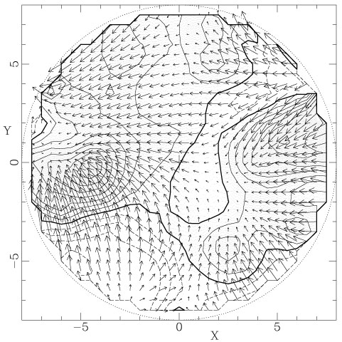
Note that the effects of items (i) and (iii) are minimized with different weightings; one can never minimize both simultaneously. In practice, the effects of these sources of noise and biases for any given dataset and smoothing scheme are calculated using extensive Monte-Carlo simulations. First results of the POTENT technique are presented in Bertschinger et al. (1990) , using the Mark II data. The resulting density field, smoothed with a 1200 km s^-1 Gaussian window, clearly shows the Great Attractor, and the void in the foreground of the Pisces-Perseus supercluster. The smoothed velocity field and resulting density field as gained from the Mark III data () are shown in Fig. 17.

Figure 17. The smoothed velocity field and resultant density field from the Mark III data, in the Supergalactic Plane. The smoothing used was a 1200 km s-1 Gaussian. The arrows give the X-Y components of the three-dimensional velocity field, while the contours are of assuming 0 = b = 1, spaced at intervals of 0.2.

The POTENT method and results have been used for a number of other studies, now using the Mark III data described in Section 7.2. We have already referred to its use to trace the density field at low Galactic latitudes (Section 3.8), and to compare the velocity fields as traced by elliptical and spiral galaxies separately (Section 6.2). Seljak & Bertschinger (1994) have used a maximum-likelihood method to fit the amplitude of fluctuations in the Mark II POTENT density field, assuming a given power spectrum. The analysis is complicated by the fact that data points are coupled not just by real correlations, but also by noise, necessitating a full Monte-Carlo approach to the covariance matrix. A summary of their results for a range of plausible CDM-like models is

(210)

where _{8, v} is the rms value of ^. v in spheres of radius 8 h^-1 Mpc. This result is in good agreement with standard CDM, normalized to the COBE quadrupole.

7.5.1. The Initial Density Distribution Function

In Section 5.2.2, we described a method developed by Nusser & Dekel (1993) which uses the Zel'dovich approximation to reconstruct the initial density distribution function from the eigenvalues of the spatial derivatives of the velocity field. It can be shown that this reconstruction is independent of ₀ when reconstructing from the velocity field predicted from a redshift survey, while the reconstruction from the observed velocity field is ₀-dependent; in particular, the shape of the derived initial density distribution function will depend on the value of ₀ used. Nusser & Dekel (1993) carried out a preliminary analysis of the Mark II POTENT velocity field using this technique, and found that they needed values of ₀ close to unity in order to match the Gaussian distribution function seen in the reconstruction from the density field. That is, for small values of ₀, the distribution function reconstructed from the observed density and velocity fields did not agree at all. Nusser & Dekel (1993) used this approach to rule out ₀ < 0.3 models at the 4-6 confidence level; the data are consistent with ₀ = 1. Further tests are needed, however, to test whether very low ₀ models, in which the derived errors become large, can be ruled out as well. The Mark III data should give much superior results.

7.5.2. Higher-Order Moments of the Velocity Field

In linear perturbation theory with Gaussian initial conditions, we saw that the density field showed a Gaussian distribution. Given the direct proportionality between and ^. v (Eq. 30), will also have a Gaussian distribution. However, just as the distribution of develops skewness in second-order perturbation theory, so does . Bernardeau (1994a, b; cf. Bouchet et al. 1993) calculates the higher-order moments of in perturbation theory for top-hat smoothing (cf. Bernardeau et al. 1994 and Lokas et al. 1994 for Gaussian smoothing), and shows that the ratio of the skewness to the variance squared is given by:

(211)

(compare with Eq. 124; like that result, this is valid only in the range -3 ₁ < 1). Unlike the case of the density field, the skewness of the velocity field is strongly dependent on ₀. Unlike the density-velocity comparisons discussed below, galaxy biasing does not affect the results (at least for equal volume weighting). Bernardeau et al. (1994) have made a tentative measurement of the skewness of the POTENT density field from the Mark III data, and conclude that the data are consistent with ₀ = 1, with ₀ = 0.3 ruled out at the 2 level. Because the skewness is so heavily weighted by the tails of the distribution, and the substantial sources of errors and biases in POTENT will strongly affect these tails, this result remains tentative, and will require extensive Monte-Carlo simulations to test it thoroughly. Higher-order moments remain unmeasurable from current data.

7.5.3. Voids in the Reconstructed Density Field

The dimensionless density field has a firm lower limit, -1, corresponding to the absence of matter. In linear theory, is proportional to the divergence of the velocity field , which says that also has a lower limit, depending only on the proportionality constant f (₀). Comparison with lowest observed point in the POTENT maps thus puts a lower limit on f (₀), again independent of galaxy biasing. Dekel & Rees (1994) have applied this idea to the Sculptor Void seen in the Mark III POTENT data (cf., Fig. 6), and find that ₀ > 0.3 at the 2.4 level. The systematics of this method have not yet been properly treated, however. In particular, as there is a strong correlation between _galaxies and , the voids that one wants to use for this test are in those regions where there are fewest galaxies, and thus the noise in the POTENT maps are highest. In addition, these are regions which potentially suffer from strong inhomogeneous Malmquist bias, precisely because the galaxy density field shows strong gradients in voids.

7.5.4. Other Approaches to Reconstructing the Velocity Field

The POTENT approach can be thought of as a parameterized fit to the velocity field, in which the velocity field in each smoothing volume is fit to a bulk flow (plus shear terms; cf. the discussion in Dekel et al. 1994). An alternative approach is to expand the velocity field in Fourier modes. Kaiser & Stebbins (1991) and Stebbins (1994) use a Bayesian approach, regularizing their solution for the Fourier coefficients by assuming that the velocities are drawn from a Gaussian distribution with a given power spectrum. Indeed, this regularization is equivalent to applying a Wiener filter to the data, and thus has the same feature as we saw above in Section 3.7: the derived density field goes to zero in regions of poor data. The results they get are a strong function of the power spectrum assumed; we await a detailed exposition of their technique in refereed journals.

As a Method I technique (Table 3) the POTENT method has the serious drawback that it assumes an a priori distance indicator relation, calibrated independently of the data in question. A small error in the slope of the Tully-Fisher relation, for example, will cause systematic errors in the derived velocity field. An alternative approach is to solve simultaneously for the parameters of the distance indicator relation and the velocity field, in a Method II approach. In the first paper that takes into account all the selection effects in such a problem, Han & Mould (1990) fit the Aaronson et al. (1982) peculiar velocity data to a model involving infall into the Virgo cluster and the Great Attractor (cf., Faber & Burstein 1988). We describe a generalization of their technique in Section 8.1.3 using the IRAS predicted velocity field.

Nusser & Davis (1994b) suggest an expansion of the radial velocity field in spherical harmonics and radial spherical Bessel functions. They find linear combinations of the basis functions that are orthonormal at the positions of the galaxies for which data exist, allowing them to find an analytic solution for the Tully-Fisher parameters and the coefficients of these orthonormalized functions as measured in redshift space by minimizing the scatter in the inverse Tully-Fisher relation (thereby eliminating selection bias). Small-scale noise and triple-valued zones eliminate the one-to-one mapping between real space and redshift space, causing a bias in the derived velocity field, although this seems to be a small effect with real data. This offers an alternative method to smooth peculiar velocity data, and may be the ideal way to compare with the predicted velocity field from redshift surveys using the Nusser & Davis (1994a) approach (cf., Davis & Nusser 1995). The applicability of the derived velocity field to points other than those where data exist remains unclear, and the method is limited to data characterized by a single distance indicator relation (or at least is analytic only in this limit). These problems are not fatal by any means, and this method holds great promise.

³¹ On large scales, these flows are referred to as as "large-scale streaming motions," "large-scale flow," "bulk flow," among other terms. We use all these terms interchangeably here. Back.

³² Willick (unpublished) has shown, however, that the limited sky coverage of the Aaronson et al. sample means that its ruling out of large-scale bulk flows is not definitive. Back.

³³ The very small Virgo infall amplitude found by FB88 remains controversial. Tonry et al. (1992) have applied the SBF technique to local ellipticals and found an infall velocity of 340 ± 80 km s^-1 at the LG. Work on the subject will undoubtedly continue in the coming years. Back.

³⁴ Colless (1995) derives a more accurate version of Eq. (200); his reanalysis of their data gives results differing only slightly from those of Lauer & Postman (1994) . Back.