


This chapter will discuss quantitative measures of galaxy clustering, and how we might use the results to put constraints on cosmological models for structure formation. Much of the background material has been introduced earlier in Section 2, although we will find ourselves introducing new concepts as we go along. We are not exhaustive in this section, and do not attempt to describe every statistic that has been used as a measure of galaxy clustering. In particular, we do not survey the work done with multi-fractal measures or percolation methods; these approaches have been thoroughly reviewed in this journal by Borgani (1995) .
We start with a discussion of the two-point correlation function
 (r) in
Section 5.1. Before going onto the power spectrum in
Section 5.3, we discuss the effects of redshift space
distortions and non-linear effects in Section 5.2.
Non-linear effects give non-zero high-order correlations, which we
discuss in Section 5.4 and
Section 5.5. Topological
measures of large-scale structure are discussed in
Section 5.6.
(r) in
Section 5.1. Before going onto the power spectrum in
Section 5.3, we discuss the effects of redshift space
distortions and non-linear effects in Section 5.2.
Non-linear effects give non-zero high-order correlations, which we
discuss in Section 5.4 and
Section 5.5. Topological
measures of large-scale structure are discussed in
Section 5.6.
The dipole moment of the galaxy distribution is closely related to the motion of the Local Group (Section 5.7). One can expand the density distribution in higher-order multipoles as well, as discuss in Section 5.8. We return to the subject of redshift-space distortions with methods to correct for them in Section 5.9. We finish this chapter with a discussion of the relative distribution of different types of galaxies, in Section 5.10.
5.1. The Two-Point Correlation Function
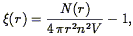
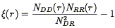
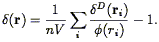
The two-point correlation function was introduced in Eq. (44) as the autocorrelation function of the (continuous) density field. As it is the Fourier Transform of the power spectrum P(k) (Eq. 46), it also gives a complete statistical description of the density field to the extent that the phases are random. Although one can always define a smoothed density field as described in Section 3.7, and then apply Eq. (44), the resulting correlation function would be cut off on scales smaller than the smoothing length. Instead, we simply apply Eq. (45), which we rewrite as follows: the joint probability that galaxies be found at positions r1 and r2 within the infinitesimal volumes V1 and V2 is

| (81) |
where
r12 = |r1 -
r2|. In the case of a volume-limited sample
(
 1) we thus find
| (82) |
where N(r)r is the number of pairs found in the
sample with separations between r and r + r, and
4  r2
rn2V is the
number expected in a uniform distribution of galaxies. This expression
is appropriate only for the case of a volume-limited sample of
galaxies, and ignores edge effects. In practice then, one does the
following
(Davis & Peebles
1983b):
one generates on the computer a
sample of points with no intrinsic clustering, but with the same
selection criteria as those of the real galaxies. Thus the mock catalog
matches the true catalog in the solid angle coverage and in the
selection function. One then counts pairs with separation between r
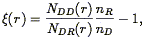
and r + r both in the real data (call this quantity
NDD(r),
with D standing for data), and between the real data and the mock
catalog (NDR(r), with R standing for
random). The correlation
function is then estimated as:
r2
rn2V is the
number expected in a uniform distribution of galaxies. This expression
is appropriate only for the case of a volume-limited sample of
galaxies, and ignores edge effects. In practice then, one does the
following
(Davis & Peebles
1983b):
one generates on the computer a
sample of points with no intrinsic clustering, but with the same
selection criteria as those of the real galaxies. Thus the mock catalog
matches the true catalog in the solid angle coverage and in the
selection function. One then counts pairs with separation between r
and r + r both in the real data (call this quantity
NDD(r),
with D standing for data), and between the real data and the mock
catalog (NDR(r), with R standing for
random). The correlation
function is then estimated as:
| (83) |
where nD and nR are the mean number densities of galaxies in the data and random samples. One usually makes the number of random galaxies much larger than that of the real sample so that additional shot noise is not introduced. In general, one can weight the pair counts any way one wants:
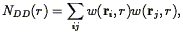
| (84) |
with a similar equation for NRR, where the sum is over
pairs of galaxies at positions ri and
rj such that
r < |ri - rj| <
r + r. For flux-limited samples, weighting by the
inverse of the product of selection functions for the two galaxies
gives equal volume weighting.
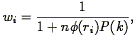
Saunders,
Rowan-Robinson, & Lawrence (1992)
show that the variance in
(r) is
minimized for the weights:
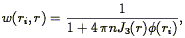
| (85) |
where J3(r) was defined above (Eq. 62). Note that Eq. (85) bears a resemblance to the minimum variance weights for the mean density, Eq. (61).
The accuracy of Eq. (83) is limited by the accuracy of the
estimate of the mean number density of galaxies; one cannot measure
(r) on scales
beyond that on which it falls below the fractional
uncertainty in the mean density of the sample. The mean density is
uncertain due to the possibility of large-scale structure on the scale
of the survey itself. That is, one never knows the extent to which a
given volume is a fair sample of the universe. The rms fluctuations
in the density on the scale of a survey are given by
Eq. (37), but of course, in order to estimate
this, we need to know P(k), which is what we are trying to
find in the first place. However, there exist estimators of
(r) whose
sensitivity to uncertainties in the mean density is appreciably weaker
than that of Eq. (83)
(Landy & Szalay
1993
;
Hamilton 1993b).
In particular,
Hamilton (1993b)
shows that the fractional error in the estimator:
| (86) |
is proportional to the square of the fractional error in the
mean density. This advantage of Eq. (86) over
Eq. (83) actually only holds for weighting
w(ri)  1 /
(ri);
otherwise, the two estimators give quite similar
results. In any case, the differences between the two become apparent
only on very large scales, where the correlation function is quite weak.
1 /
(ri);
otherwise, the two estimators give quite similar
results. In any case, the differences between the two become apparent
only on very large scales, where the correlation function is quite weak.
There has been a great deal of confusion over the proper estimation of the error in the correlation function. There are two sorts of statistical error one could try to calculate:
Many of the analyses in the literature consider only one of these two effects. The problem is inherently difficult because the variance in the two-point correlation function necessarily depends on the three- and four-point correlation functions (to be discussed in Section 5.4). In addition, there exists strong covariance between the estimate of the correlation function on different scales, which of course is strongest for estimates at two closely spaced scales.
Peebles (1973)
and Kaiser (1986)
calculate the shot noise contribution to the correlation function errors
in terms of a cluster model: if we think of the galaxy distribution as
a smooth field with clusters embedded, the number of galaxies
associated with each cluster is
1 + 4 nJ3
(we restrict ourselves for the
moment to the case of a volume-limited sample). The number of
independent pairs of galaxies at a given separation is the number of
observed pairs, NDD, divided by the number associated
with the
clusters. That is, because galaxies are clustered, a majority of the
galaxy pairs are redundant. The resulting error in the correlation
function is then just given by Poisson statistics:
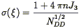
| (87) |
Kaiser (1986)
notes that
NDD  n2, and thus for
4 nJ3 >> 1,
n2, and thus for
4 nJ3 >> 1,
 () is independent of
n. Thus he argues that
given a finite amount of telescope time, one wants to sparse-sample to
the level that
4 nJ3
() is independent of
n. Thus he argues that
given a finite amount of telescope time, one wants to sparse-sample to
the level that
4 nJ3
 1 (i.e., roughly one
galaxy per
cluster), maximizing the volume covered to minimize the effect of
power on scales larger than the sample. This is a meaningful strategy,
if in fact one's primary motivation is to measure
(r) on large
scales. This is the motivation behind the 1-in-6
sampling of the QDOT survey
(Lawrence et al. 1994),
and the 1-in-20 sampling of the APM survey
(Loveday et al. 1992a
b).
1 (i.e., roughly one
galaxy per
cluster), maximizing the volume covered to minimize the effect of
power on scales larger than the sample. This is a meaningful strategy,
if in fact one's primary motivation is to measure
(r) on large
scales. This is the motivation behind the 1-in-6
sampling of the QDOT survey
(Lawrence et al. 1994),
and the 1-in-20 sampling of the APM survey
(Loveday et al. 1992a
b).
Ling, Frenk, &
Barrow (1986)
argue that the effect of shot noise can
best be estimated by making bootstrap realizations of a given sample,
and calculating the scatter in the determination of
(r) from each
of these. Although the mean
(r) over the
bootstraps is unbiased,
this results in an overestimation of the errors, as shown by
Mo, Jing, & Börner (1993)
and Fisher et
al. (1994a) .
Fisher et al. (1994a)
describe a brute-force way to make realistic estimates
of the correlation function error covariance matrix: make a series of
independent N-body realizations of a given sample, and calculate the
scatter of the estimates of
(r) from each
of these. Of course,
this estimate will be only as good as the power spectrum assumed for
the simulation itself, although it is probably not terribly sensitive
to the details. Existing redshift surveys are not large enough to be
able to afford to split the surveys up into pieces and compute errors
from the variance in the estimated correlation function in each,
although
Hamilton (1993b)
describes a practical method to estimate
correlation function errors from one's dataset itself, by considering
the contribution that each subvolume in a sample makes to the
correlations.
The two-point correlation function can be applied not only to redshift
data, but also to surveys containing only angular data. The
angular correlation function can be defined in analogy with
Eq. (81): the joint probability that galaxies be found
at angular positions
 1 and
2 within
the infinitesimal solid angles
d
1 and
2 within
the infinitesimal solid angles
d 1 and
d2 is
1 and
d2 is
| (88) |
where
 12 is the angle
between 1 and
2, and
12 is the angle
between 1 and
2, and
 is the number density of
galaxies on the sky.
Groth & Peebles
(1977)
calculated the angular correlation function of
the Shane-Wirtanen Lick galaxy counts (cf., the beginning of
Section 4); they found that
w() is
well fit by a power law of slope 0.77 for scales smaller than about
2°, with a sharp break on larger scales (cf, the challenge to
their results by
Geller, Kurtz, & de
Lapparent (1984)
and de Lapparent,
Kurtz, & Geller (1986)
over the issue of plate matching). More
recently, the angular correlation function of the APM galaxies has
been calculated by
Maddox et al. (1990a)
,
who reproduce the
Groth & Peebles
(1977)
results on small scales; however, the APM correlation function breaks
on a somewhat larger scale than that of the Lick counts. The APM data
are of higher photometric accuracy than the Lick data, and because the
catalog was generated automatically it is immune from the inevitable
systematic effects that counting galaxies by eye entails. Other recent
determinations of the angular correlation function include
Picard (1991)
and
Collins, Nichol, &
Lumsden (1992) .
Bernstein (1994)
has carried out a detailed analytic analysis of the error in the angular
correlation function (using the estimator of
Landy & Szalay
1993),
including the covariance terms, and using the hierarchical hypothesis
(Eq. 120) to include the effects of three-point and
four-point correlations. The resulting expressions are too complicated
to reproduce here, but do an excellent job of matching the errors
measured from Monte-Carlo simulations.
is the number density of
galaxies on the sky.
Groth & Peebles
(1977)
calculated the angular correlation function of
the Shane-Wirtanen Lick galaxy counts (cf., the beginning of
Section 4); they found that
w() is
well fit by a power law of slope 0.77 for scales smaller than about
2°, with a sharp break on larger scales (cf, the challenge to
their results by
Geller, Kurtz, & de
Lapparent (1984)
and de Lapparent,
Kurtz, & Geller (1986)
over the issue of plate matching). More
recently, the angular correlation function of the APM galaxies has
been calculated by
Maddox et al. (1990a)
,
who reproduce the
Groth & Peebles
(1977)
results on small scales; however, the APM correlation function breaks
on a somewhat larger scale than that of the Lick counts. The APM data
are of higher photometric accuracy than the Lick data, and because the
catalog was generated automatically it is immune from the inevitable
systematic effects that counting galaxies by eye entails. Other recent
determinations of the angular correlation function include
Picard (1991)
and
Collins, Nichol, &
Lumsden (1992) .
Bernstein (1994)
has carried out a detailed analytic analysis of the error in the angular
correlation function (using the estimator of
Landy & Szalay
1993),
including the covariance terms, and using the hierarchical hypothesis
(Eq. 120) to include the effects of three-point and
four-point correlations. The resulting expressions are too complicated
to reproduce here, but do an excellent job of matching the errors
measured from Monte-Carlo simulations.
The angular correlation function
w() for a
flux-limited sample is related to the spatial correlation function by
Limber's (1953)
equation (cf.
Rubin 1954):
| (89) |
where is the
selection function,
r12
|r1 - r2|, and
is the angle between
r1 and r2.
It is straightforward to show from Eq. (89) that a
power-law spatial correlation function of logarithmic slope
 corresponds to an angular correlation function with logarithmic slope
- 1. Thus we expect the
spatial correlation function to be a power law with slope
= 1.77, at least on small
scales. The
spatial correlation function has been determined for essentially all
the large redshift surveys discussed above in
Section 3.1; important papers include
Davis & Peebles
(1983b)
,
Bean et al. (1983)
,
Shanks et al. (1983)
,
Davis et al. (1988)
,
de Lapparent, Geller,
& Huchra (1988)
,
Strauss et al. (1992a)
,
Fisher et al. (1994a)
,
Moore et al. (1994)
, and
Loveday et al. (1995)
.
Because of
the much smaller number of galaxies included in redshift surveys than
in the angular catalogs, the spatial correlation function is
determined with lower accuracy on large scales. However, these studies
and others have demonstrated convincingly that the spatial correlation
function is indeed a power-law on small scales, with a break at
approximately 2000 km s-1. The much quoted relation of
Davis & Peebles
(1983b)
,
corresponds to an angular correlation function with logarithmic slope
- 1. Thus we expect the
spatial correlation function to be a power law with slope
= 1.77, at least on small
scales. The
spatial correlation function has been determined for essentially all
the large redshift surveys discussed above in
Section 3.1; important papers include
Davis & Peebles
(1983b)
,
Bean et al. (1983)
,
Shanks et al. (1983)
,
Davis et al. (1988)
,
de Lapparent, Geller,
& Huchra (1988)
,
Strauss et al. (1992a)
,
Fisher et al. (1994a)
,
Moore et al. (1994)
, and
Loveday et al. (1995)
.
Because of
the much smaller number of galaxies included in redshift surveys than
in the angular catalogs, the spatial correlation function is
determined with lower accuracy on large scales. However, these studies
and others have demonstrated convincingly that the spatial correlation
function is indeed a power-law on small scales, with a break at
approximately 2000 km s-1. The much quoted relation of
Davis & Peebles
(1983b)
,
| (90) |
is consistent with the observed power-law behavior of
w().
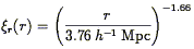
Eq. (90) also
implies that the rms galaxy fluctuations within spheres of radius 8
h-1 Mpc are unity
(Eq. 37) (16) .
This is a scale below which the clustering
is clearly strongly non-linear, and much of the formalism developed in
Section 2.2 becomes irrelevant.
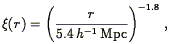
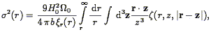
A primordial power spectrum of power law slope greater than zero implies that P(0) = 0. It then follows from Eq. (46) that the volume integral of the spatial correlation function over all of space must be zero, meaning that the correlation function must go negative at some point. Given a power spectrum, for example, that of Standard Cold Dark Matter, one can use Eq. (46) to predict that the correlation function goes negative on scales above 33 h-1 Mpc, and reaches a minimum at 46 h-1 Mpc with an amplitude of -1.5 × 10⁻³. This is too small an effect to have been measured in any existing galaxy sample. Indeed, if one defines the mean density of a sample from the sample itself (as is usually done), the integral of the correlation function over the volume of the survey is forced to zero. This effect tends to bias the correlation function low, at least when it is estimated for small volumes.
The power-law nature of the correlation function has prompted some
workers to suggest that galaxies follow a fractal distribution, with
no preferred scale (e.g.,
Coleman & Pietronero
1992). In such a
model, it would not be possible to define a mean density of the
universe; it would be a function of the scale on which one measured
it. However, the correlation function is defined in terms of
 , which has the mean density
subtracted already. The correlation function of
1 + predictably is
not scale-free (e.g.,
Guzzo et al. 1991
;
Calzetti, Giavalisco,
& Meiksin 1992).
Peebles (1993)
shows that
the observed scaling of the angular correlation function with depth
rules out simple fractal models (cf.
Davis et al. 1988).
More complicated, multi-fractal models have been proposed; they are
reviewed thoroughly in
Borgani (1995).
, which has the mean density
subtracted already. The correlation function of
1 + predictably is
not scale-free (e.g.,
Guzzo et al. 1991
;
Calzetti, Giavalisco,
& Meiksin 1992).
Peebles (1993)
shows that
the observed scaling of the angular correlation function with depth
rules out simple fractal models (cf.
Davis et al. 1988).
More complicated, multi-fractal models have been proposed; they are
reviewed thoroughly in
Borgani (1995).
5.2. Distortions in the Clustering Statistics
The next logical topic to discuss would be the determination of the power spectrum of the galaxy distribution. Before we do so, however, we outline the principal effects which cause the observed correlation function and power spectrum to differ from those which held following the epoch of radiation-matter equality, extrapolated via linear theory to the present. These are:
We will discuss the redshift space distortions and the non-linear effects here.
5.2.1. Redshift Space Distortions
The effect of peculiar velocities on the shape of structures can be understood heuristically by imagining the gravitational influence of a rich cluster of galaxies. On small scales, within the virialized cluster itself, galaxies have peculiar velocities of 1000 km s-1 or more, which causes a characteristic stretching of the redshift space distribution along the line of sight. This is called the " Finger of God", which points directly at the origin in a redshift pie diagram; the Finger of God associated with the Coma cluster is apparent in Fig. 3. Thus a compact configuration of galaxies is stretched out along the line of sight, greatly reducing the correlations: the small-scale velocity dispersion of galaxies causes the correlation function to be underestimated in redshift space.
On larger scales, a different effect operates: galaxies outside the cluster itself feel the gravitational influence of the cluster, and thus have peculiar velocities falling into it. A galaxy on the far side of the cluster will thus have a negative radial peculiar velocity, and appear closer to us in redshift space than in real space, while a galaxy on the near side will have a positive peculiar velocity, and appear further away from us. Thus the gravitational influence of a cluster causes a compression of structures, thus enhancing the correlation function.
These two effects can be quantified. The effect of the large-scale motions can be calculated via linear theory, as was first done in the present context by Kaiser (1987; cf. Sargent & Turner 1977). In brief, one calculates the change in the Jacobian of the volume element in going from real to redshift space. The result is that in linear theory, both the power spectrum and correlation function are enhanced in redshift relative to their real space counterparts by a factor:
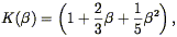
| (91) |
where  was defined above in
Eq. (51). For = 1, K =
1.87, so this is not a small effect. This calculation is
done in the "distant observer approximation", in which the volume
surveyed is supposed to subtend a small angle from the point of view
of the observer. For further discussion of this approximation, see
Cole, Fisher, & Weinberg (1994)
,
and Zaroubi &
Hoffman (1994).
was defined above in
Eq. (51). For = 1, K =
1.87, so this is not a small effect. This calculation is
done in the "distant observer approximation", in which the volume
surveyed is supposed to subtend a small angle from the point of view
of the observer. For further discussion of this approximation, see
Cole, Fisher, & Weinberg (1994)
,
and Zaroubi &
Hoffman (1994).
One way to disentangle the effects of peculiar velocities from true
spatial correlations is to divide the vector separating any two
galaxies into components in the plane of the sky (rp
in the notation of
Fisher et al. 1994a),
and along the line of sight
(). The effects of redshift space
distortions are purely radial,
and thus the correlation function projected onto the plane of the sky
is a measure of the real space correlation function. In practice,
then, we measure
s as a
function of both rp and
. The
subscript s reminds that this is a quantity measured in redshift
space. The projection of s(rp,
) onto the rp
axis yields
a quantity closely related to the angular correlation function
(Davis & Peebles
1983b):
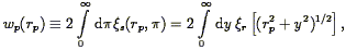
| (92) |
where here r
is the desired real space correlation function, as
indicated by the subscript r. For a power-law correlation function
r(r)
= (r / r0)-, the integral can be done
analytically, yielding
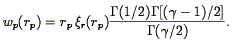
| (93) |
This is the approach that Davis & Peebles (1983b) took to find the result in Eq. (90); Fisher et al. (1994a) used this method to find
| (94) |
for IRAS galaxies.
Saunders,
Rowan-Robinson, & Lawrence (1992)
measured
r(r)
for IRAS galaxies using a related approach: they
cross-correlated the QDOT redshift survey with its parent 2D catalog
(Rowan-Robinson et
al. 1991)
to suppress the redshift spacing
distortions; they find results in excellent agreement with Eq. (94) (cf.
Loveday et al. 1995
for a measurement of
the APM correlation function using the same technique). The
significance of the discrepancy in the amplitudes and slopes between
the IRAS (Eq. 94) and optical
(Eq. 90) correlation functions will be discussed in
Section 5.10.
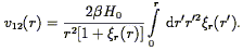
If we could measure the Kaiser effect of Eq. (91)
directly, we could constrain the parameter
. The difficulty is
that Eq. (91) is only valid on large scales where linear
theory is valid, and where the competing effect of small-scale
velocity dispersion is unimportant. But of course, the correlations
are small and difficult to measure on these large scales.
Gramann, Cen, &
Bahcall (1994)
and Brainerd &
Villumsen (1994)
point out that
if the small-scale velocity dispersion were as large as predicted by
standard CDM, then the Kaiser effect would be swamped by the
suppression of the correlation function due to the velocity dispersion
until one gets to truly enormous scales. Nevertheless, several groups
have attempted to measure the Kaiser effect directly from redshift
survey data.
Fry &
Gaztañaga (1993)
compared the correlation function measured in
redshift space for various redshift surveys to the angular correlation
function of the same samples (which are free from redshift space
distortions). They found
= 0.53 ± 0.15
for the CfA survey,
= 1.10 ± 0.16 for the
SSRS, and = 0.84 ± 0.45
for the IRAS 1.936 Jy survey. Alternatively, one
looks for the anisotropy of
s(rp,
) in the radial and
transverse directions.
Hamilton (1992)
defines the angular moments of the correlation function as
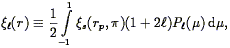
| (95) |
where P is the
th Legendre
polynomial and
µ is the cosine of the angle between the line of sight and the
redshift separation vector. He then shows that:
is the
th Legendre
polynomial and
µ is the cosine of the angle between the line of sight and the
redshift separation vector. He then shows that:
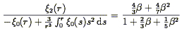
| (96) |
in the linear regime.
Hamilton (1993a)
applies this to the IRAS 1.936 Jy sample to find
=
0.69+0.28-0.24.
Fisher et al. (1994b)
took a somewhat different approach,
including the effects of both the small-scale velocity dispersion and
large-scale Kaiser effect, and fitting directly to
s(rp,
).
Following
Peebles (1980)
,
the relation between the
real and redshift space correlation functions can be written as

| (97) |
where the integral is over possible values of the radial peculiar
velocity difference w3, and f
(w3| r) is the distribution function
of w3 at a given separation r. An exponential
distribution is a good approximation to the distribution function found
in N-body simulations;
Fisher et al. (1994b)
show that it gives a better fit
than does a Gaussian to the real data. Taking the shape of the first
and second moments of f as a function of r from
N-body models,
Fisher et al. were able to reduce the model-fitting to two free
parameters: the amplitude of the second moment
(i.e., the
pairwise velocity dispersion) at
r = 100 km s-1, and the amplitude of
the first moment v12 (i.e., the mean pairwise
streaming of galaxies) at
r = 1000 km s-1. They show, in analogy with
Eq. (91), that linear theory predicts the following form
for the first moment:
| (98) |
Thus the measurement of
v12 = 109+64-47 km
s-1 at 1000 km s-1,
together with the real-space correlation function
(Eq. 94), directly yields a value for
; they find
=
0.45+0.27-0.18. Although this statistic is shown
to be unbiased with the help of N-body simulations, its power is
limited by the volume of the sample. We assume that any anisotropy
measured in the sample is due to redshift-space distortions, but the
real space correlation function will be isotropic only to the extent
that the sample includes enough volume to average over the orientation
of elongated superclusters.
It is not a priori obvious that the approach of writing the effect of the redshift space distortions as a convolution with the velocity distribution function (Eq. 97) is consistent with linear theory in the form of Eq. (91); linear theory predicts covariance between the velocity and density fields that is not included in Eq. (97). However, Fisher (1995) has been able to reproduce Eq. (91) by expanding Eq. (97) to second order, assuming that f (w| r) is Gaussian, with mean value and dispersion as given by linear theory.
The Fisher et
al. (1994b)
analysis also measures the distortions on
non-linear scales to derive the pair-wise velocity dispersion at 100
km s-1,
=
317+40-49 km s-1. This is
to be compared with the
Davis & Peebles
(1983b)
value of
340 ± 40 km s-1 from the CfA
survey, also measured by looking at redshift space
distortions (17) .
The predicted values of
for different power spectra (as calculated with N-body simulations)
are quite different, so this quantity is of great interest for
constraining models. High resolution dissipationless simulations of
Standard CDM indicate
~ 1000 km
s-1 for the dark matter (e.g.,
Davis et al. 1985
;
Gelb & Bertschinger
1994b),
far in excess
of what is observed. However, this number has been controversial: it
is the velocity dispersions of galaxies, not dark matter particles,
which are observed. The velocity dispersion of halos of dark
matter particles in simulations
(Brainerd &
Villumsen 1993;
Gelb & Bertschinger
1994)
are smaller than that of the dark matter itself,
although these simulations suffer from the so-called over-merging
problem, in which groups of galaxies merge in enormous supergalaxies,
which have no counterparts in the real world. Because
is
weighted by pairs of galaxies, such over-merging tends to cause the
estimate of to be biased
low. Hydrodynamical simulations of
CDM, which tend to avoid the over-merging problem, radiatively
dissipate some of the energy that would otherwise go into galaxy
motions, and in fact find a lower value for
(e.g.,
Cen & Ostriker
1993),
although still not low enough to match the observed value above.
Weinberg (1994)
shows that the velocity dispersion is
very sensitive to the details of the biasing model used to define
galaxies from the distribution of dark matter.
Velocity dispersion analyses of other redshift surveys
(Mo et al. 1994)
show a larger for some
samples, although the pair-weighting nature of
makes it quite
sensitive to a few rare clusters in a survey volume
(Zurek et al. 1994).
What is needed to settle this controversy is a new statistic
which is less weighted by the rare high velocity-dispersion clusters,
and thus more strongly reflects the velocity dispersion in the field.
The small-scale velocity dispersion can also be used to apply the Cosmic Virial Theorem (Peebles 1976a , b; Peebles 1980): if one assumes statistical equilibrium of clustering on small scales, and takes the continuum limit, one can show that
| (99) |
where  is the
three-point correlation function, to be discussed
in Section 5.4. This equation can be simplified
assuming a hierarchical model for the three-point correlation function
(Eq. 118), and a power-law form for the two-point
correlation function (Eq. 75.14 of
Peebles 1980).
In practice, the
application of this equation is hampered by our poor knowledge of the
three-point correlation function. More importantly, the linear biasing
model assumed in Eq. (99) is questionable at
best on these very inhomogeneous scales. Finally,
Carlberg, Couchman,
& Thomas (1990)
argue that galaxies may not be fair tracers of the velocity
field on small scales, a form of velocity bias. The
Cosmic Virial Theorem has been used to argue for a small value of
is the
three-point correlation function, to be discussed
in Section 5.4. This equation can be simplified
assuming a hierarchical model for the three-point correlation function
(Eq. 118), and a power-law form for the two-point
correlation function (Eq. 75.14 of
Peebles 1980).
In practice, the
application of this equation is hampered by our poor knowledge of the
three-point correlation function. More importantly, the linear biasing
model assumed in Eq. (99) is questionable at
best on these very inhomogeneous scales. Finally,
Carlberg, Couchman,
& Thomas (1990)
argue that galaxies may not be fair tracers of the velocity
field on small scales, a form of velocity bias. The
Cosmic Virial Theorem has been used to argue for a small value of
 0 =
0.2e±0.4
(Davis & Peebles
1983b),
but if dark matter is not clustered with galaxies on the very small
scales of 100 km s-1, Eq. (99) will return an underestimated
value of 0
(Bartlett &
Blanchard 1994).
0 =
0.2e±0.4
(Davis & Peebles
1983b),
but if dark matter is not clustered with galaxies on the very small
scales of 100 km s-1, Eq. (99) will return an underestimated
value of 0
(Bartlett &
Blanchard 1994).
Cole, Fisher, & Weinberg (1994) take a parallel approach to Hamilton (1992; 1993a), based on the power spectrum. Just as we can separate the vector between two galaxies into parallel and perpendicular components, we can separate a wave vector k into parallel and perpendicular components, if we work with a subsample of a survey with small total opening angle with respect to the observer, the distant observer approximation discussed above. In analogy with Eq. (95), they define angular moments of the power spectrum:
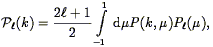
| (100) |
and show that the rational expression in Eq. (96)
can be expressed as
 2(k) /
0(k). Applying this to
the 1.2 Jy IRAS redshift survey, they find
= 0.35 ± 0.05,
although they emphasize that non-linear effects cause this to be a
lower limit. A recent re-analysis by
Cole, Fisher, &
Weinberg (1995)
parameterizes the effects of non-linearity in the velocity field by
including a small-scale velocity dispersion in their model, in analogy
to the analysis by
Fisher et al. (1994b)
. They find
= 0.52 ± 0.13 for the
IRAS 1.2 Jy sample, and
= 0.54 ± 0.3 for the
QDOT survey.
2(k) /
0(k). Applying this to
the 1.2 Jy IRAS redshift survey, they find
= 0.35 ± 0.05,
although they emphasize that non-linear effects cause this to be a
lower limit. A recent re-analysis by
Cole, Fisher, &
Weinberg (1995)
parameterizes the effects of non-linearity in the velocity field by
including a small-scale velocity dispersion in their model, in analogy
to the analysis by
Fisher et al. (1994b)
. They find
= 0.52 ± 0.13 for the
IRAS 1.2 Jy sample, and
= 0.54 ± 0.3 for the
QDOT survey.
As in all these methods,
non-linear effects have the potential to break the degeneracy between
0 and
b. Non-linear effects make the effective value of
as derived from this method
grow as a function of scale until
the linear regime is reached; the scale at which the curve asymptotes
is thus a measure of the strength of the mass clustering, and
can be used to put constraints on the bias parameter. Unfortunately,
existing redshift surveys are not extensive enough to measure this
effect with confidence.
In linear perturbation theory, the real space density field differs from the primordial density field only by a universal scaling factor. However, this is no longer true when non-linear effects become important. There has been a great deal of work in recent years on non-linear extensions to Eq. (30) (Bernardeau 1992a ; Gramann 1993a ; Nusser et al. 1991 ; Giavalisco et al. 1993 ; Mancinelli & Yahil 1994 ; cf. Mancinelli et al. 1994 for a comparison of these techniques), and various approximate non-linear schemes to bridge the gap between linear theory and N-body simulations (Peebles 1989a , 1990, 1994; Weinberg 1991 ; Matarrese et al. 1992 ; Brainerd, Scherrer, & Villumsen 1993 ; Bagla & Padmanabhan 1994). Here we wish to concentrate on methods to take redshift surveys back in time to their initial conditions. Weinberg (1989; 1991) adopts the assumption that the initial density distribution function is Gaussian, and notes that the rank order of densities is likely to be preserved even as non-linear effects skew the distribution function. Thus he applies a technique called Gaussianization, whereby the rank order of the densities at different points is conserved, but the densities are reassigned to fit a Gaussian form. The details of this method depend on assumptions about galaxy biasing and the power spectrum. The idea is to apply the Gaussianization technique to redshift survey data, measure the power spectrum of the resulting density field, and then evolve the resulting initial conditions forward in time again using an N-body code. To the extent that the assumed and measured power spectra match, and the final results agree with the original data, one has demonstrated consistency with the input model. Weinberg (1989) applied this technique on a volume-limited subsample of the Pisces-Perseus survey of Giovanelli & Haynes (1988) . The power spectrum was consistent with that of standard CDM. Unbiased models did not work, not reproducing the filamentary structure of the real data; b = 2 was a better match to the real data. Most importantly, the analysis tests, and finds consistency, with the assumptions of Gaussian initial conditions and gravitational instability.
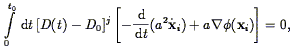
Nusser & Dekel (1992) have developed a time machine to take the observed density field (as derived from a redshift survey or the POTENT method; cf. Section 7.5 below) back in time. The equations of motion allow a decaying mode (Eq. 26), which gets amplified if one simply reverses the density evolution equations. Nusser & Dekel (1992) instead start with the Zel'dovich equation (Eq. 34), which when expressed in Eulerian coordinates yields a first-order differential equation for the velocity potential which only allows a growing mode:
| (101) |
where  v
is the potential associated with the scaled velocity field
v v /
a
v
is the potential associated with the scaled velocity field
v v /
a 1. This
Zel'dovich-Bernoulli equation
can be integrated backwards in time from observations of the density
fields; N-body tests show the results to reproduce the initial
conditions better than does linear theory.
1. This
Zel'dovich-Bernoulli equation
can be integrated backwards in time from observations of the density
fields; N-body tests show the results to reproduce the initial
conditions better than does linear theory.
Gramann (1993a) shows that consideration of the continuity equation in the context of the Zel'dovich equation yields a correction term Cg to the right hand side of Eq. (101), given by:
| (102) |
where g
is the gravitational potential. N-body tests show
this equation reproduces the non-linear evolution better than does
Eq. (101), although this approach has not
been applied to redshift surveys yet.
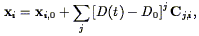
Nusser & Dekel (1993) have used the Zel'dovich approximation in another version of their time machine. Assuming laminar flow, one can write down the eigenvalues of the space derivatives of the initial velocity field in Lagrangian space in terms of the eigenvalues of the space derivatives of the observed velocity field in Eulerian space ðvi / ðxi. Assuming further that linear theory holds in the initial conditions (as it should), one can derive the initial density field via Eq. (30); the final result is
| (103) |
where D is the time dependence of the growing mode of gravitational instability (Eq. 27). They use the IRAS 1.936 Jy redshift survey and the methods of Section 5.9 to generate the predicted velocity field and thus the initial density field, from which they determine the initial density distribution function. They find it to be accurately Gaussian. Application of their technique to the observed velocity field is described in Section 7.5.1.
Another approach to non-linear gravitational evolution was taken by Peebles (1989a; 1990), and amplified by Giavalisco et al. (1993) . One can derive the exact equations of motion for a multi-body gravitating system by finding the stationary points of the action S:
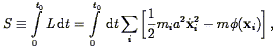
| (104) |
where the sum is over the particles in the system, mi
are their masses, xi are their comoving positions, and
is the
gravitational potential. Giavalisco et al. then expand the positions
xi in a Taylor series, of which the Zel'dovich equation
(Eq. 34) is the first two terms:
| (105) |
where the Cj,i are coefficients to be determined. Setting the derivative of the action S with respect to the Cj,i yields the set of equations
| (106) |
which can be solved for the unknowns Cj,i. This method is exact except in regions in which multi-streaming has occurred, that is, where a single point in Eulerian space corresponds to more than one point in Lagrangian space. Giavalisco et al. (1993) have tested this approach against spherical infall models, and show that it converges very quickly. Peebles (1989a; 1990) has used this method in the analysis of the dynamics of the Local Group, and the first attempts to extend this method to redshift surveys can be found in Peebles (1994) , and Shaya, Peebles, & Tully (1994) .
Hamilton et al. (1991)
have taken an empirical approach to non-linear
evolution of the power spectrum. Considerations of galaxy conservation
within a radius r0 fixed in Lagrangian space around a
galaxy in an
0 = 1 universe
yields the hypothesis that the quantity
a2J3(r0) /
r03 is invariant with time, where
J3 is given by
Eq. (62). Tests with N-body models show this in fact to be
the case, and that this quantity is independent of the initial power
spectrum, allowing the initial correlation function to be read off
that measured. Using this method on the IRAS, CfA, and APM
correlation functions allowed them to reproduce the initial
correlation function, which they found to be best fit by a model
invoking a mix of cold and hot dark matter. Extensions of their method
can be found in
Peacock & Dodds
(1994)
,
discussed further below, and
Mo, Jain, & White
(1995) .
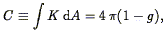
In principle, the correlation function should contain all the information about the power spectrum, given that the two are a Fourier Transform pair (Eq. 46). However, there are two strong reasons to calculate the power spectrum directly from redshift surveys:
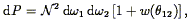
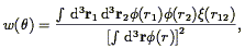
The power spectrum can be calculated from a galaxy redshift survey as follows. The unsmoothed density field is given by a sum over Dirac delta functions:
| (107) |
Taking the Fourier Transform of this yields
| (108) |
where
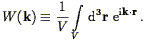
| (109) |
Our estimator of the power spectrum is then

| (110) |
where the factor of V on the right hand side gets the units right. Several lines of algebra (Fisher et al. 1993) show that the expectation value of this estimator is given by
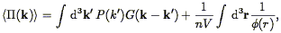
| (111) |
where
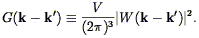
| (112) |
Thus the power spectrum estimator is given by the true power spectrum convolved with an expression involving the Fourier Transform of the volume, plus a shot noise term. In the limit of an infinitely large volume, G approaches a Dirac delta function.
The power spectrum as so defined is a function of the direction of
k. In practice, one averages
< (k)> over 4
steradians in k-space.
Fisher et al. (1993)
introduce the trick of
measuring the power spectrum within cylinders embedded within the
survey volume, whose long axis of length 2R is parallel to the
vector k. If one then chooses
kR = n with n
a positive integer, the window function W vanishes
(Eq. 109). This has two benefits:
(k), and
therefore the power spectrum now scale exactly with mean density, and
thus errors in the mean density affect only the amplitude, and
not the shape, of the power spectrum. In addition, the values of
the power spectrum at different values of k are uncorrelated;
there is no covariance between them.
(k)> over 4
steradians in k-space.
Fisher et al. (1993)
introduce the trick of
measuring the power spectrum within cylinders embedded within the
survey volume, whose long axis of length 2R is parallel to the
vector k. If one then chooses
kR = n with n
a positive integer, the window function W vanishes
(Eq. 109). This has two benefits:
(k), and
therefore the power spectrum now scale exactly with mean density, and
thus errors in the mean density affect only the amplitude, and
not the shape, of the power spectrum. In addition, the values of
the power spectrum at different values of k are uncorrelated;
there is no covariance between them.
Feldman, Kaiser, &
Peacock (1994)
have taken a slightly different approach. They include a weight function in
Eq. (108), and derive an expression for the
variance in the power spectrum estimator, assuming that the error
distribution of P(k) is exponential (which follows from a
Gaussian distribution of
(r)). Minimizing the
ratio of this
variance to P2 gives the optimum weight function for
galaxy i:
| (113) |
which is of a similar form to the optimum weight for the mean density (Eq. 61) and the correlation function (Eq. 85). With this weight function, the variance in the estimate of the power spectrum is given by
| (114) |
where Vk is the volume in k-space occupied by
the bin in
question. This expression assumes that the bins are spaced far enough
apart that the covariance is negligible (this happens roughly for
separations
 k > 2
/ R, where R is the
characteristic dimension of the volume surveyed). They also derive an
expression for the off-diagonal terms of the covariance matrix; see
their paper for details.
k > 2
/ R, where R is the
characteristic dimension of the volume surveyed). They also derive an
expression for the off-diagonal terms of the covariance matrix; see
their paper for details.
The power spectrum of galaxies has been calculated for a number of
redshift surveys
(Baumgart & Fry 1991
;
Peacock & Nicholson
1991
;
Park, Gott, & da Costa 1992,
Vogeley et al. 1992
;
Fisher et al. 1993
,
Feldman et al. 1994;
Park et al. 1994
;
da Costa et al. 1994b;
Lin 1995).
Although there is reasonable agreement in the literature now
about the shape of the power spectrum on small scales, its amplitude,
especially on large scales, remains uncertain. The data are consistent
with a slope of
P(k)
k-1.4 on small scales, and several authors (e.g.,
da Costa et al. 1994b)
show an abrupt change of slope at
2 / k = 50
h-1 Mpc. All theoretical power spectra show a turnover
on scales of 100 h-1 Mpc or more
(Fig. 2); this has not
yet been seen unequivocally in the data. A number of authors
(Peacock 1991
;
Torres, Fabbri, &
Ruffini 1994
;
Kashlinsky 1992
;
Branchini, Guzzo, &
Valdarnini 1994
;
Padmanabhan &
Narasimha 1993 )
have derived
empirical power spectra to fit the various data sets. The most
thorough of these analyses is that of
Peacock & Dodds
(1994)
,
who have combined a number of the above datasets, together with the
real-space correlation function (from the angular correlation function;
Baugh & Efstathiou
1993 ).
They correct each for the Kaiser
effect (Eq. 91) on large scales, and the effects of
small-scale velocity dispersion, following
Peacock (1991) .
Moreover, they correct for non-linear effects using the approach of
Hamilton et al. (1991)
(Section 5.2.2), extending the formalism to the
0
1 case. They combine the
different samples, asking for
consistency while adjusting five free parameters: four bias values
(for Abell clusters, radio galaxies, optical galaxies, and IRAS
galaxies), plus 0,
which determines the strength of the
Kaiser effect (Eq. 91). They find that
00.6 /
bIRAS = 1.0 ± 0.2. The small errors on this
number imply that the redshift space distortion is unambiguously
detected, largely based on the comparison with the real-space
correlation function of
Baugh & Efstathiou
(1993) .
The constraint on
bIRAS separately is less strong, but is consistent
with unity. The ratios of the various bias factors are:

| (115) |
Their results on the reconstructed linear power spectrum are shown in
Fig. 9. The points are means of the power spectrum
from the various data sets, for
0 =
bIRAS = 1. The two
curves are standard CDM (dashed), and
 = 0.25 CDM, normalized
to the power spectrum implied by the CMB anisotropies as measured by
the COBE satellite (indicated by the box on the left-hand side of the
figure). The data are clearly far more consistent with the
= 0.25 CDM model than with
standard CDM, both in amplitude and in
shape (indeed, Peacock & Dodds come to this conclusion without
consideration of the normalization afforded by the COBE data). This
result is consistent with the conclusions of a number of workers in
the field; we discuss the issues further in
Section 9.1.
= 0.25 CDM, normalized
to the power spectrum implied by the CMB anisotropies as measured by
the COBE satellite (indicated by the box on the left-hand side of the
figure). The data are clearly far more consistent with the
= 0.25 CDM model than with
standard CDM, both in amplitude and in
shape (indeed, Peacock & Dodds come to this conclusion without
consideration of the normalization afforded by the COBE data). This
result is consistent with the conclusions of a number of workers in
the field; we discuss the issues further in
Section 9.1.

|
Figure 9. The power spectrum as derived
from a variety of redshift
surveys, after correction for non-linear effects, redshift
distortions, and relative biases; from
Peacock & Dodds
(1994) .
The two curves show the Standard CDM power spectrum, and that of CDM with
|
The second moment of the density distribution function is directly related to the power spectrum via Eq. (37). It can be calculated directly from redshift surveys as the second moment of the count distribution function (after correction for shot noise; cf., Peebles 1980 ; Saunders et al. 1991), and thus represents another handle on the power spectrum itself. This has been done by Efstathiou et al. (1990) , Saunders et al. (1991) , Loveday et al. (1992a) , Bouchet et al. (1993) , and Moore et al. (1994) , among others; the results they find are consistent with those shown in Fig. 9. A compilation of second moment results for IRAS galaxies is shown in Fisher et al. (1994a) . It makes the qualitative point that the variance drops as the scale increases, as is required by the Cosmological Principle, and follows for any power spectrum with n > - 3 (Eq. 39).
As we have mentioned above, the power spectrum, or its Fourier
Transform, the two-point correlation function, is a complete
statistical description of the density field
only to the
extent that the phases of the Fourier modes of
are random,
implying that the one-point distribution function of the density
field is Gaussian. Even if this condition holds for the density field
in the early universe (as is predicted by inflationary models), it
begins to break down as soon as non-linear effects start to
develop. We discussed theoretical approaches to this problem in
Section 5.2.2. In this and the following section,
we discuss methods of measuring these non-linear effects from the data.
One can obviously extend the definition of the two-point correlation function to higher order. We can define the three-point correlation function for the continuous density field as

| (116) |
However, the practical definition in terms of the point distribution is more complicated, because of the need to correct for the contribution due to the fact that galaxies have a two-point correlation function. In analogy to Eq. (81), the probability of finding galaxies at distinct positions r1, r2, and r3 within volume elements V1, V2, and V3 is:
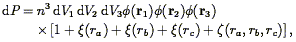
| (117) |
where ra, rb and
rc are the sides of the triangle defined by
the three points. One can immediately see the difficulty in measuring
, as it requires
subtracting four terms from the triple counts.
In addition, the three-point correlation function is now a function of
three numbers, not just one. The problem only gets worse for
higher-order correlation functions; the equivalent expression to
Eq. (117) for the four-point correlation function has
fifteen terms on the right hand side (Eq. 35.1 of
Peebles 1980).
Despite these difficulties, the three- and four-point
correlation functions have been measured for the Shane-Wirtanen counts
(Fry & Peebles 1978
;
Fry 1983
;
Szapudi, Szalay, &
Boschan 1992),
the CfA redshift survey
(Bonometto & Sharp
1980;
Gaztañaga 1992),
and the IRAS samples
(Meiksin, Szapudi,
& Szalay 1992
;
Bouchet et al. 1993).
These samples have measured non-zero three- and four-point
correlation functions on small scales, indicating that the phases are
indeed not random. More importantly, they have shown that the three-
and four-point correlation functions display a certain symmetry with
respect to the two-point correlation function:

| (118) |
where Q is independent of scale and triangle configuration, to the
level that the data can distinguish these things. In particular, there
are no "loop terms", proportional to
(ra)
(rb)
(rc),
which puts strong constraints on the form of biasing (e.g.,
Szalay 1988).
A similar expression
holds for the four-point correlation function. It has therefore been
hypothesized that Eq. (118) can be generalized to the
Nth order correlation function, indicated as
N (not to
be confused with the of
Eq. 95!).
Balian & Schaeffer
(1989)
assume that the N-point
correlation function shows scale invariance:

| (119) |
for any  . They show that
this allows one to write
. They show that
this allows one to write
| (120) |
where the constants SN uniquely define the hierarchical scaling, and the correlation functions averaged over a sphere are given by:
| (121) |
This volume-averaging integrates over the shape information in the
high-order correlation function. Although there is much that can be
learned from the dependence of the high-order correlations on the
angles between the N points
(Suto & Matsubara
1994
;
Fry 1994),
the volume-averaged statistic is much more robust for small
datasets. Moreover, the
 N(V) are
equal to the irreducible
Nth-order moments of the density distribution
function: the skewness is
3(V) =
<3>, the
kurtosis is
4(V) =
<4> -
3<2>, and
so on
(Peebles 1980).
For a power-law correlation function, the relation
between (r)
and its volume average can be calculated analytically
(Peebles & Groth
1976):
N(V) are
equal to the irreducible
Nth-order moments of the density distribution
function: the skewness is
3(V) =
<3>, the
kurtosis is
4(V) =
<4> -
3<2>, and
so on
(Peebles 1980).
For a power-law correlation function, the relation
between (r)
and its volume average can be calculated analytically
(Peebles & Groth
1976):
| (122) |
There has been a great deal of interest in recent years to calculate
the hierarchy of SN, both from the theoretical and
observational
sides. The use of volume averaging mitigates the need to calculate the
N-point correlation function with its dependence on
N(N - 1)/2
separations. In practice, one calculates the moments
µN of the
galaxy count distribution function, which are then corrected for
shot-noise effects following Section 36 of
Peebles (1980; cf.
Szapudi & Szalay
1993
;
Gaztañaga &
Yokohama 1993)
to yield
N. This only
works for volume-limited samples, or
angular data; flux-limited samples require a more elaborate correction
(Saunders et al. 1991).
One can then compare the observations with the predicted
scaling, Eq. (120). As we will see momentarily, this
scaling holds remarkably well, giving support to the scale invariant
hypothesis (Eq. 19).
However, Eq. (19), or equivalently,
Eq. (120), seems to have been pulled out of a hat.
Before we show the observational evidence for them, let us discuss
their theoretical motivation. For initial conditions with random
phases, all SN for N
 3 are zero initially. However, as
clustering grows and becomes non-linear, the density distribution
function becomes non-Gaussian, and higher-order moments become
non-zero.
Peebles (1980)
first calculated the skewness (i.e., third
moment) of the unsmoothed density field in second-order
perturbation theory for an
0 = 1 universe,
and showed that
3 are zero initially. However, as
clustering grows and becomes non-linear, the density distribution
function becomes non-Gaussian, and higher-order moments become
non-zero.
Peebles (1980)
first calculated the skewness (i.e., third
moment) of the unsmoothed density field in second-order
perturbation theory for an
0 = 1 universe,
and showed that

| (123) |
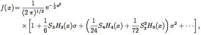
in agreement with Eq. (120). However, observationally, we are always limited to the smoothed density field, for which the quantity S3 depends on the power spectrum (Juszkiewicz, Bouchet, & Colombi 1993):
| (124) |
where µ is the cosine of the angle between k and k', W is the Fourier Transform of the window (cf. Eq. 38), and
| (125) |
where the derivative is calculated at the smoothing scale.
Eq. (124) is valid for -3  1 < 1.
The
calculations get more difficult for increasing N; calculation of
SN requires the application of N - 1-order
perturbation theory. One
can show straightforwardly, however, that in every case, the scaling
of Eq. (120) holds
(Fry 1984a ,
b;
Bernardeau 1992b).
In a mathematical tour-de-force,
Bernardeau (1994b)
has set up a formalism
for calculating the SN for all N for a tophat
window function,
and presents expressions up to N = 7 as a function of the
i, I>i = 1,
..., N. It turns out that it is more difficult
mathematically to do the calculations for Gaussian smoothing, although
the cases N = 3
(Juszkiewicz et
al. 1993)
and N = 4
(Lokas et al. 1994)
have analytic solutions. Analogous calculations have been done
for the non-linear evolution of the power spectrum by
Juszkiewicz (1981)
,
Makino, Sasaki, &
Suto (1992)
,
Jain & Bertschinger
(1994)
and others.
Feldman et al. (1994)
examine the cumulative distribution function of
|2(k)| in
the QDOT data, and show it to be accurately exponential,
as expected in a Gaussian field. However, the expected distribution in
the mildly non-linear regime in the presence of shot noise has not yet
been calculated.
1 < 1.
The
calculations get more difficult for increasing N; calculation of
SN requires the application of N - 1-order
perturbation theory. One
can show straightforwardly, however, that in every case, the scaling
of Eq. (120) holds
(Fry 1984a ,
b;
Bernardeau 1992b).
In a mathematical tour-de-force,
Bernardeau (1994b)
has set up a formalism
for calculating the SN for all N for a tophat
window function,
and presents expressions up to N = 7 as a function of the
i, I>i = 1,
..., N. It turns out that it is more difficult
mathematically to do the calculations for Gaussian smoothing, although
the cases N = 3
(Juszkiewicz et
al. 1993)
and N = 4
(Lokas et al. 1994)
have analytic solutions. Analogous calculations have been done
for the non-linear evolution of the power spectrum by
Juszkiewicz (1981)
,
Makino, Sasaki, &
Suto (1992)
,
Jain & Bertschinger
(1994)
and others.
Feldman et al. (1994)
examine the cumulative distribution function of
|2(k)| in
the QDOT data, and show it to be accurately exponential,
as expected in a Gaussian field. However, the expected distribution in
the mildly non-linear regime in the presence of shot noise has not yet
been calculated.
The results quoted thus far are for an
0 = 1 universe in
real
space. The dependence of the SN on
0 is extremely weak
(Bouchet et al. 1992
,
1994),
and is also insensitive to the transformation
from real to redshift space. Moreover, it can be shown that the
scaling relations Eq. (120), continue to hold under
arbitrary local biasing transformations (Eq. 50),
although the values of the SN themselves change
(Fry &
Gaztañaga 1993
;
Juszkiewicz et al. 1995
;
Fry 1994).
Biasing models which are non-local,
in which the probability that a galaxy be formed at a given point is a
function of events removed by tens of Mpc from that point, have been
invoked to explain the mismatch of the observed power spectrum with
Standard CDM (e.g.,
Babul & White 1991
;
Bower et al. 1993).
However, such models break the scale-invariant hierarchy by adding loop
terms (e.g.,
Szalay 1988), and
Frieman &
Gaztañaga (1994)
have used the excellent agreement with the scale-invariant predictions
(e.g., Fig. 10) to rule
out a wide class of these models.
The calculation of S3 and S4 has been done for the CfA and SSRS samples (Gaztañaga 1992) and the IRAS 1.2 Jy sample (Bouchet et al. 1993), as well as for various angular catalogs (Szapudi, Szalay, & Boschan 1992 ; Meiksin, Szapudi, & Szalay 1992 ; Gaztañaga 1994 ; Szapudi et al. 1995). All these authors have found beautiful agreement with the predicted scaling relation: the results from the IRAS survey are shown in Fig. 10. Gaztañaga (1994) finds that the value of S3 varies slightly with scale; this is expected by Eq. (124) if the power spectrum is not a pure power law. Inserting the power spectrum for the APM counts of Baugh & Efstathiou (1993) in Eq. (124) gives beautiful agreement with the observed values, implying that the biasing is very weak. This conclusion depends on the biasing being linear; non-linear biasing can mimic absence of biasing in the dependence of S3 on scale.
|
Figure 10. The skewness (upper panel) and the kurtosis (lower panel) of the IRAS density field for various smoothing lengths, as a function of the variance. The plots are logarithmic. The lines drawn are least-square fits, with slopes 1.96 ± 0.06, and 3.03 ± 0.18, respectively. This figure is taken from Bouchet et al. (1993) . |
Thus the scaling relations Eq. (120) were originally
hypothesized on largely aesthetic grounds. They were found to be
predicted by perturbation theory assuming Gaussian initial conditions,
and growth of structure via gravitational instability. Indeed,
calculations of the skewness in initially non-Gaussian models
(Fry & Scherrer
1994
;
Bouchet et al. 1994)
show that the leading behavior goes like
23/2,
rather than
22 as
observed. May we therefore conclude that we can rule out non-Gaussian
models? Unfortunately, the answer is no. First, the
23/2
term decays with time, and at late times, may be
negligible. Moreover, as many have quipped, referring to non-Gaussian
models is a little like referring to non-elephant animals; the range
of possible non-Gaussian models is vast. Weinberg & Cole (1992) set
up a series of non-Gaussian models by skewing the density distribution
function of an initially Gaussian model, but the resulting
non-Gaussianity exists only on the smoothing scale on which
is defined. On scales appreciably larger than this, the Central Limit
Theorem guarantees that the distribution is Gaussian again, and
the scaling laws between the various moments will continue to
hold. Thus one needs to examine each specific non-Gaussian model in
turn, ask for its predictions for the scaling either using analytic
techniques or N-body simulations
(Moscardini et al. 1991
;
Weinberg & Cole
1992),
and compare with the data. This process has not been
carried out in detail at this writing.
Finally, Fig. 10 shows that the scaling relation between the moments predicted by second-order perturbation theory holds well into the highly non-linear regime, where it has no right to hold (although this has been a working hypothesis for the closure of the so-called BBGKY equations; cf., Davis & Peebles 1977). Similar behavior has been seen in N-body simulations (e.g., Juszkiewicz et al. 1994). There is controversy about the effect of redshift space distortions in these analyses: Lahav et al. (1993a) , Suto & Matsubara (1994) , and Matsubara & Suto (1994) argue on the basis of N-body simulations that redshift space distortions make the SN closer to constant than in real space in the non-linear regime, a conclusion supported by the analytic calculations of Matsubara (1994a) , and the observations of the Pisces-Perseus region by Ghigna et al. (1994) . However, Fry & Gaztañaga (1993) find that the SN are remarkably constant in both redshift and real space on small scales, in a variety of redshift surveys. In any case, there exists no analytic argument as to why hierarchical scaling should hold into the non-linear regime.
5.5. The Density Distribution Function and Counts in Cells
One of the striking features of the galaxy distribution is the presence of voids as much as 6000 km s-1 in diameter. The statistical tools that we have presented thus far do not clearly indicate their presence; we see no feature in the correlation function on such scales. Thus we look for a statistic that is more specifically oriented to describing the visible structures that we see. One such statistic is the void probability function. Imagine laying down a series of spheres of radius r randomly within a large volume populated with galaxies. Define the void probability function P0(r) as the fraction of those spheres which contain no galaxies. In the absence of clustering, Poisson statistics yields

| (126) |
where n is the mean density of galaxies and
V = 4
r3/3 is
the volume of a sphere. In the clustered case, P0
depends on the whole hierarchy of correlation functions, as shown by
White (1979)
:

| (127) |
where the volume-averaged correlation functions were introduced in Eq. (121). Thus the void probability function is a complementary statistic to the correlation functions. One can compute not only P0, but also the probability of observing N galaxies within a sphere; it is related to P0 as:
| (128) |
The void probability function is clearly a strong function of the
sparseness of a given sample, and thus masks to a certain extent the
underlying galaxy distribution. One way around this is to define a
sampling independent quantity  :
:
| (129) |
so that a Poisson distribution gives
= 1
(Eq. 126). If the hierarchical hypothesis
Eq. (120) holds, then Eq. (127) implies
that is
a universal function, independent of the sampling; indeed, this is
observed for the IRAS galaxies
(Bouchet et al. 1993
,
but see
Vogeley et al. 1991).
(r) is observed to be a
smooth monotonically decreasing curve
with no features; no particular scale is picked out.
The void probability function is potentially a useful discriminant of cosmological models. However, Weinberg & Cole (1992) and Little & Weinberg (1994) found that the void probability function is insensitive to the power spectrum or the density parameter, and is more sensitive to the details of the biasing scheme than to the bias value itself.
Under the scale-invariant hypothesis (Eq. 19), one can make quite detailed predictions for the form of the PN (Balian & Schaeffer 1989). Indeed, the density distribution function is given by (cf. Bernardeau & Kofman 1995):
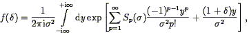
| (130) |
which is an exact expression to the extent that the Sp are exact (18) . The PN follow from this after convolving with a Poisson distribution to include the effects of shot noise.
The various predictions developed by Balian & Schaeffer (1989) based on the scale-invariant hypothesis have been checked in N-body simulations (Bouchet et al. 1991; Bouchet & Hernquist 1992), although very dense sampling is required to test the full suite of predictions. The PN have been derived observationally for various data sets (Alimi, Blanchard, & Schaeffer 1990 ; Maurogordato, Schaeffer, & da Costa 1992 ; Lahav & Saslaw 1992; Bouchet et al. 1993). The latter authors compare the observed counts in cells with various models, and find that a range of models (including those of Carruthers & Shih 1983 ; Saslaw & Hamilton 1984 ; Coles & Jones 1991) become degenerate at the sparse sampling of existing surveys, and the data cannot distinguish between them.
Another approach to the density distribution function (which is just
PN(r) at constant r) was introduced by
Juszkiewicz et
al. (1995) .
On large scales, where the second moment of the
distribution function
2
<2> is
small, the
deviation of the distribution function from a Gaussian is expected to
be small. Thus it makes sense to expand the distribution function in
orthogonal polynomials relative to the Gaussian. The Edgeworth
expansion does this:
| (131) |
where the HN(x) are the Hermite polynomials, and
x = /
. This is found to give an
excellent fit to the
distribution function in N-body models for small
, although for
0.5 the Edgeworth expansion
starts going unphysically
negative at moderate values of x. Maximum-likelihood calculations of
SN using fits of Eq. (131) to the observed
PN may
be more robust than calculation of the moments directly. Indeed, the
results of the moments method are heavily weighted by the tails of the
distribution. This is dangerous when working within a finite volume,
because one is sensitive to the rare dense clusters
(Colombi, Bouchet,
& Schaeffer 1994
,
1995
We motivated this section by pointing out that standard correlation statistics do a poor job of quantifying the largest scale features that are apparent to the eye in redshift maps. The void probability function goes part of the way in filling this need, although it is not as discriminating a statistic between different cosmological models as was hoped. There have been a number of papers discussing various statistics to capture the largest-scale features apparent in the redshift maps (Tully 1986 , 1987a Broadhurst et al. 1990 ; Babul & Starkman 1992 , although again the robustness of these statistics, and their discriminatory power, have been questioned (Postman et al. 1989 ; Kaiser & Peacock 1991 . One of the most successful statistics to describe large-scale structure in a way complementary to correlation functions uses concepts from topology, to which we now turn.
5.6. Topology and Related Issues
What is the mental picture we should have of the topology of the
galaxy distribution? Is it a uniform sea of galaxies punctuated by
rich clusters embedded in it, like meatballs in a bowl of spaghetti?
Dramatic voids are what catch the eye in
Fig. 3; would a
better picture be a uniform distribution with voids scooped out of it,
like a piece of swiss cheese? If the density distribution is Gaussian,
then there should in fact be a topological symmetry between underdense
and overdense regions, like a piece of sponge. Motivated by these
considerations,
Gott, Melott, &
Dickinson (1986)
,
who are responsible
for these food analogies, suggested measuring the topology of the
galaxy isodensity surfaces. In particular, given a surface in
three-space, one can define the principal radii of curvature
a1 and
a2 at every point. By the Gauss-Bonnet theorem, the
integral of the Gaussian curvature
K 1 /
a1a2 over the surface is given by
| (132) |
where g is the genus number of the surface (the number of holes
minus the number of disjoint pieces, plus 1). Thus measurements of the
Gaussian curvature give the genus of the surface. A plot of genus of
the isodensity surface as a function of density thus tells us the
change in the topology at different contrast levels. What do we expect
in the Gaussian model? At very high density contrasts, the isodensity
contours will surround isolated clusters, and thus the genus will be
negative. Similarly, for
close to -1, the isodensity
contours will surround isolated voids, and again the genus will be
negative. The mean isodensity contour will be multiply connected and
sponge-like, and thus have a positive genus. One can calculate
analytically the genus number in the Gaussian case
(Doroshkevich 1970
;
Bardeen et al. 1986
;
Hamilton, Gott, &
Weinberg 1987
;
cf. Coles 1988
for specific non-Gaussian models):
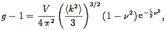
| (133) |
where V is the volume of the survey,
 =
/
is the level of the density
in units of the rms of the density field,
=
/
is the level of the density
in units of the rms of the density field,
| (134) |
is the second moment of the smoothed power spectrum, and
W(k) is the
Fourier Transform of the smoothing window. Measurements of the genus
as a function of thus
characterize the general topology of the
density field. In particular, we can test the Gaussian hypothesis by
comparing the observed form to Eq. (133). To the
extent that the observed genus curve is well-fit by the Gaussian form,
the amplitude of the curve is a measure of the shape of the power
spectrum at the wavelength of the smoothing. The amplitude of
the power spectrum cancels out of Eq. (134). Gott and
collaborators use a volume-weighting technique to reduce the
sensitivity of the topology statistic to non-linear evolution and to
separate the topological information from that carried by the density
distribution function. Calculations
of the genus curve from redshift surveys have been carried out by
Gott et al. (1989),
Moore et al. (1992)
, and
Vogeley et al. (1994)
,
using a tessellation technique for measuring the genus number
(Gott et al. 1986;
cf. Weinberg 1988
for the source code). Unfortunately, the volume of existing surveys is
small, and thus for smoothing lengths in the linear regime, the
maximum genus levels are ~ 20. The results show a slight
"meatball" shift relative to the Gaussian case; that is, the
overdense contours show larger values of g than
Eq. (133) would predict. This is in the sense
expected from non-linear evolution
(Matsubara 1994b).
The amplitude
of the genus curve as a function of smoothing scale is in rough
agreement with that predicted by CDM, although
Moore et al. (1992)
find some evidence for power in excess of CDM predictions on large
scales. Statistical errors of the measurement of genus are usually
calculated using bootstrap techniques, although these suffer from the
same drawback as bootstraps for correlation functions
(Section 5.1). At the moment, there is no rigorous
error analysis
of the genus statistic, nor any calculation of the effects of shot
noise (which will tend to make the distribution function look more
Gaussian). Very recently,
Matsubara (1995)
has studied the effect of
redshift space distortions on the genus statistic.
A related statistic was invented by Ryden (1988) : the area of the isodensity surfaces. For a Gaussian field, one again expects a symmetric function, which again peaks at the mean density. The area is given by
| (135) |
Ryden et al. (1989) invented a clever technique to measure this statistic, involving counting how often skewers put randomly through the survey volume intersect the isodensity surface, and applied this to the CfA survey and the Giovanelli & Haynes Perseus-Pisces survey. At 1200 km s-1 Gaussian smoothing, the results closely matched the linear theory predictions. At 600 km s-1 smoothing, however, the data showed stronger deviations from Gaussianity than did any of the models examined. However, their models were probably not evolved forward to become sufficiently non-linear on 600 km s-1 scales; this remains a problem for further investigation.
One of the early motivations behind redshift surveys of the full sky
was to apply Eq. (33) to the Local Group. The CMB
shows a dipole anisotropy of amplitude
T / T
10-3
(Kogut et al. 1993,
and references therein), which is interpreted as a
Doppler effect due to the motion of the earth relative to the rest
frame of the last scattering surface. When transformed to the
barycenter of the Local Group following
Yahil et al. (1977),
this motion is 627 ± 22 km s-1 towards
l = 276 ± 3°,
b = + 30 ± 3° (Galactic coordinates). Given a full-sky
redshift
survey, a comparison of this motion with the dipole moment of the
galaxy distribution is a direct measure of
. In fact, because
both gravity and received light obey the inverse-square law, if one
assumes a constant mass-to-light ratio for the galaxies, there is a
direct proportionality between the peculiar velocity and the ratio of
the dipole and monopole moments of the light distribution, allowing
Eq. (33) to be applied using angular data only
(Gott & Gunn 1973).
The angular dipole moment of the galaxy distribution has been measured by a
number of authors using a variety of galaxy catalogs
(Meiksin & Davis
1986
;
Yahil, Walker, &
Rowan-Robinson 1986
;
Villumsen & Strauss
1987
;
Lahav 1987
;
Harmon, Lahav, &
Meurs 1987
;
Lahav, Rowan-Robinson,
& Lynden-Bell 1988
;
Plionis 1988
;
Lynden-Bell, Lahav,
& Burstein 1989
;
Kaiser & Lahav 1989
;
Scharf et al. 1992).
The first
impressive result of these analyses is that the vector direction of
the light dipole agrees with that of the CMB dipole to within
10 - 30°, depending on the specific sample and analysis used.
There is greater disagreement in the amplitude of the dipole, with
results varying from
= 0.3 to
= 1.2.
Rather than discuss the details of this here, let us move to the
application of Eq. (33) using redshift surveys.
The first measurement of the gravitational dipole from a redshift
survey was by
Davis & Huchra
(1982)
,
using a combination of the CfA and Revised Shapley-Ames
(Sandage & Tammann
1981)
surveys. Given the
limited sky coverage of their sample, they were able only to measure
the component of the acceleration towards the Galactic poles, which
they compared to measured Virgocentric infall
(Section 8.1.1), to find values of
(19)
ranging from 0.38 to 0.74, depending on exactly what assumptions were made.
More recently,
Pellegrini & da Costa (1990)
combined redshift survey
data from several different surveys, and carried out a similar
comparison to the Virgocentric infall; they found
in the range
0.24 to 0.56. Further progress had to await the completion of redshift
surveys of the entire sky. The dipole moment of the IRAS QDOT
redshift surveys was calculated by
Rowan-Robinson et
al. (1990)
,
who found convergence of the dipole only beyond 10,000
km s-1. The amplitude
of the dipole implied
= 0.82 ± 0.15.
Hudson (1993b)
used his reconstruction of the optical
galaxy density field to calculate the galaxy dipole; assuming that the
dipole converges within 8000 km s-1 allowed him to conclude that
=
0.80+0.21-0.13.
We cannot simply calculate the right hand side of Eq. (33) given a redshift survey. The quantity that we do calculate is the dipole moment of the galaxy distribution:
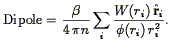
| (136) |
This differs from the dipole integral because of a number of effects, which we need to quantify:
| (137) |
Strauss et al. (1992c)
develop a maximum likelihood analysis that
allows them to take the first three of these effects into account. A
power spectrum must be assumed in the analysis in order to quantify
the effect of density fluctuations outside the assumed window. Indeed,
one can include parameters of the power spectrum in the maximum
likelihood analysis, although in practice, the constraints one can put
on models are not very strong. The rocket effect is minimized using
self-consistent solutions for the velocity field (cf.
Section 5.9). The IRAS data imply
=
0.55+0.20-0.12, where the angle between the
acceleration and velocity vectors is
18 - 25°, depending on which self-consistent
velocity field is used.
In models without large amounts of power on large scales, one expects
the dipole to converge within the volumes probed by redshift surveys;
that is, the contribution to the dipole on large scales should be
negligible. The Strauss et al. results are consistent with the dipole
converging within 4000 km s-1, although this depends on which
self-consistent density field is used, and how one corrects for the
Kaiser effect. In addition, there is a substantial dipole moment
contributed by galaxies between 17,000 and 20,000
km s-1, aligned with
the low-redshift dipole, although the sample is so sparse at those
redshifts as to make this significant at only the 2
level. If
this large additional contribution to the dipole is found at higher
significance level with deeper redshift surveys, this will imply large
amounts of power on large scales, and a smaller value of
than inferred above.
An approach to quantifying the galaxy density field complementary to correlation functions uses the method of spherical harmonics. The Fourier components of the density field that are used in the power spectrum are orthonormal within a cube. Spherical harmonics are an orthonormal set of functions on a sphere, and thus are especially appropriate for full-sky samples. They offer a natural way to smooth the data; if one expands to a given order in l, the smoothing length is an increasing function of distance from the observer, mimicking the drop-off in the sampling in a flux-limited sample.
Spherical harmonics are simply the generalization to higher
order of the dipole analysis discussed in the previous section. They
have been used for many years to describe the distribution of galaxies
in the celestial sphere, when redshift information was unavailable
(Peebles 1973
;
Peebles & Hauser
1973
,
1974;
Fabbri & Natale
1989
;
Scharf et al. 1992).
One can express the galaxy density
(,
) on the sky in
spherical harmonics as
| (138) |
where the coefficients of the observed dataset are given by
| (139) |
The sum is over the N galaxies in the sample, and the integral is
over the solid angle subtended by the sample
sample. For an
exactly full-sky sample, the second term vanishes.
The spherical harmonics can be related to the power spectrum straightforwardly. Scharf et al. (1992) show that the expectation value of the square of the coefficients in a Gaussian model with power spectrum P(k) is given by:
| (140) |
where
| (141) |
is a tensor which couples together different modes in the case of incomplete sky coverage, and the spherical harmonics in the case of complete sky coverage are given by
| (142) |
Scharf et al. (1992)
used the angular distribution of the IRAS 1.936
Jy sample to put limits on the power spectrum, parameterized by an
amplitude and a shape parameter,
0h
(Eq. 42). A maximum likelihood analysis yields
0h = 0.25,
8 = 0.8, with
remarkably tight error bars.
Scharf & Lahav (1993) have extended this analysis using the redshift information of the 1.936 Jy sample as well. Much the same formalism is used, with the addition of a redshift weighting factor f (r) in the expansion of the density field (Eq. 138). In analogy to the dipole analysis described in the previous section, the growth of all the multipole moments with redshift is used as a diagnostic of the power spectrum. The resulting constraints on the power spectrum are similar to those which Scharf et al. (1992) found from the angular data alone, although Scharf & Lahav point out that redshift space distortions are a non-negligible effect.
Fisher, Scharf, &
Lahav (1994)
have calculated these redshift space
distortions in linear theory. They find that the rms spherical
harmonic amplitudes for a full sky redshift survey (i.e.,
sample = 4
), as measured in redshift space, is
| (143) |
compare with Eq. (142). When measured for a real data
set, there is of course an additional term due to shot noise. The
dependence of Eq. (143) means
that one
can use the redshift distortions to measure
, in exact analogy
to the analyses of redshift space distortions of the correlation
function and power spectrum. Of course, the shape and amplitude of the
power spectrum also come into play; using a generic CDM spectrum
(Eq. 42),
Fisher (1994)
finds = 0.94 ± 0.17
and = 0.17 ± 0.05. A
similar analysis by
Heavens & Taylor
(1994)
yields = 1.1 ± 0.3.
5.9. Recovering the Real Space Density Field
As we have emphasized throughout this review, redshifts are not
equivalent to distances; the two differ due to peculiar velocities.
However, to the extent that peculiar velocities are due to gravity,
and that linear theory holds, we can use Eq. (33) to
estimate these peculiar velocities. Of course, this requires knowledge
of the density field, of which have a distorted view due to peculiar
velocities. Thus we look for a self-consistent solution to the density
and velocity field, given redshifts and positions for a flux-limited
redshift survey of galaxies, and assuming a value of
. In
practice, this is doable only for full-sky redshift surveys, for which
the integral in Eq. (33) can be carried out.
Yahil et al. (1991) describe an iterative technique to find this optimum solution. We describe it here in its latest incarnation (Willick et al. 1995d), as applied to the IRAS 1.2 Jy sample:
, and smoothing
with a Gaussian using
FFT's. The resulting density field is filtered with the
power-preserving filter (Section 3.7),
taking into
account the increased shot noise as a function of distance from the
origin.
(r) and velocity field
v(r)
along the line of sight  to
a given galaxy with Local Group
redshift cz and flux f, one can calculate the probability
P(r| cz, f )r that it have distance
between r and r + r:
to
a given galaxy with Local Group
redshift cz and flux f, one can calculate the probability
P(r| cz, f )r that it have distance
between r and r + r:
| (144) |
where  is the galaxy luminosity
function, v(0) is the peculiar velocity at the origin, and
v is a measure of the
small-scale velocity dispersion not included in the smooth velocity
field model. This method is inspired by the analysis discussed in
Section 8.1.3 below. If the velocity
field model were perfect,
the exponential would be replaced by a delta function at
cz = r + .
[v(r) - v(0)]; the Gaussian included here
parameterizes our ignorance
about the velocity field on scales smaller than the smoothing length.
In the presence of clusters, there are regions in which the peculiar
velocity changes with distance fast enough that one finds
triple-valued zones, in which a given redshift can correspond to
three distances. This is illustrated in Fig. 11,
which shows the relation between redshift and distance along a line of
sight which intersects a large cluster. Infall into the cluster causes
the dramatic S-curve. A galaxy at a redshift of 1200
km s-1 could lie at any of the three distances. The probability
function of Eq. (144) is shown as well; it correctly
parcels the probability among these three solutions. In particular,
the nearest crossing point is most strongly favored, given the
luminosity function weighting.
is the galaxy luminosity
function, v(0) is the peculiar velocity at the origin, and
v is a measure of the
small-scale velocity dispersion not included in the smooth velocity
field model. This method is inspired by the analysis discussed in
Section 8.1.3 below. If the velocity
field model were perfect,
the exponential would be replaced by a delta function at
cz = r + .
[v(r) - v(0)]; the Gaussian included here
parameterizes our ignorance
about the velocity field on scales smaller than the smoothing length.
In the presence of clusters, there are regions in which the peculiar
velocity changes with distance fast enough that one finds
triple-valued zones, in which a given redshift can correspond to
three distances. This is illustrated in Fig. 11,
which shows the relation between redshift and distance along a line of
sight which intersects a large cluster. Infall into the cluster causes
the dramatic S-curve. A galaxy at a redshift of 1200
km s-1 could lie at any of the three distances. The probability
function of Eq. (144) is shown as well; it correctly
parcels the probability among these three solutions. In particular,
the nearest crossing point is most strongly favored, given the
luminosity function weighting.
is incremented on each
iteration so that the effects of
peculiar velocities grow gradually, the selection function is
recalculated, and the iterations start again at step (iii) above.
This is the method used to generate Figs. 6 - 8 above. This basic approach of an iterated solution to the velocity field via Eq. (33) has been used by Yahil et al. (1991) , Strauss et al. (1992c) , Hudson (1993a, b), and Freudling et al. (1994).
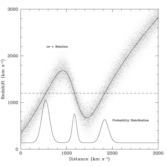
|
Figure 11. An illustration of a triple-valued zone. The S-shaped curve shows the relation between redshift and distance along the line of sight to a cluster. A galaxy with a redshift of 1200 km s-1 can lie at three distinct distances. When the small-scale noise inherent in any velocity field model, as given by the scattered points, is taken into account, the distribution function of distances for a given redshift gets smoothed out, as shown as the three-peaked curve at the bottom. |
Nusser & Davis
(1994a)
take a different approach to the problem. They
point out that the difference between the redshift and real space
position of galaxies is directly related to the displacement of a
galaxy from t = 0 to the present (the Zel'dovich approximation,
Eq. 34). Conservation of galaxies, and
the assumption that the velocity field is irrotational, allows them to
write down a Jacobian for the transformation from the initial
conditions in real space to the final configuration in redshift space,
which yields a differential equation for the velocity potential
. Expanding
and the density field
(s) in redshift
space on a given shell in spherical harmonics yields the equation:

| (145) |
where is the
selection function, and s is the redshift
coordinate. This equation can be integrated for
lm using
standard numerical techniques, and the radial velocity field can then be
derived by differentiation. This method has the advantage that it does
not require iteration (every term in Eq. (145) is in
redshift space), but because it requires a one-to-one correspondence
between real and redshift space, it does not allow the existence of
triple-valued zones.
A similar approach is taken by Fisher et al. (1995) . They decompose the density field with spherical harmonics and spherical Bessel functions for the radial component:
| (146) |
They use the fact that for a survey with full-sky coverage, redshift
space distortions couple only modes with a given l but with
different n's, but there is no coupling between different
angular modes. The coupling matrix is analytic, and its inverse allows
the real space to be
calculated from the redshift space
, one spherical harmonic at
a time. The velocity field then
follows directly from Eq. (33). In practice,
Fisher et al. (1995)
use the Wiener filter to suppress shot noise. This
method also does not require iteration.
Fisher et al. (1994d)
test the
three methods presented here with the aid of a mock IRAS 1.2 Jy
redshift survey drawn from an N-body simulation; all three give
residual rms errors in the radial peculiar velocity field in the Local
Group frame for galaxies within 6000 km s-1 of
200 km
s-1. These comparisons have only been made at the
positions of the
galaxies used in the analysis; there is a need to compare the full velocity
and density fields on a uniform grid.
Other approaches to real space reconstruction of redshift surveys include Kaiser et al. (1991) , Taylor & Rowan-Robinson (1994) , Gramann (1993b) , & Tegmark & Bromley (1994) .
5.10. Clustering of Different Types of Galaxies
Galaxy formation is a very poorly understood process. Our difficulties in understanding it stem both from our ignorance of the nature of dark matter, which presumably forms the potential wells within which the baryons that eventually form the stars of the galaxy fall, and the extreme complexity of the diverse hydrodynamic and stellar dynamic effects that become important as gas begins to radiate and stars form. In the context of this review, our principal concern is to gain some understanding of the relative distribution of the dark matter and galaxies, because it is the sum of the two which gravitates, while we can observe only the latter directly. In Section 2.4, we introduced the concept of biasing, and discussed the various contexts in which we might imagine that the distributions of galaxies and dark matter might differ. Here we ask how we might find observational evidence for biasing.
We observe that galaxies come in a variety of types, defined morphologically: from elliptical galaxies, through lenticulars, and then spirals both barred and unbarred, and finally irregulars and dwarfs of various sorts. If galaxies as a whole are biased relative to the dark matter, in the sense that the large-scale distributions of the two differ on large scales, one would expect that the process of galaxy formation caused the distribution of each of the galaxy types to be biased with respect to one another. Again, because galaxy formation is a poorly understood process, we do not have an accepted model for the Hubble sequence of morphological types, and we cannot be much more specific than this at this stage of our understanding. Nevertheless, this offers a well-posed observational problem: if we can measure biasing of one galaxy type relative to another, we have the potential of constraining biasing models.
One form of relative biasing has been known about since the time of
Hubble: the cores of rich clusters are preferentially rich in
elliptical galaxies. This was put on a firm quantitative basis by
Dressler (1980a,
b;
1984)
and Postman &
Geller (1984)
,
who showed that
the relative fraction of elliptical galaxies rose from its mean of
~ 15% in the field starting at overdensities of
~ 200, to nearly unity in
the highest-density regions of
clusters. This means that redshift maps of elliptical galaxies in
redshift surveys look qualitatively very different from those of
spiral galaxies: the clusters are much more prominent in the former (cf.
Giovanelli et al. 1986;
Huchra et al. 1990a).
This dramatic
segregation of ellipticals and spirals does not extend into the field,
but subtle relative biasing on large scales between the two have not
yet been ruled out.
A number of workers have looked for such effects in the correlation
statistics
(Davis, Geller, &
Huchra 1978
;
Giovanelli, Haynes,
& Chincarini 1986
;
Santiago & da Costa
1990
;
Einasto 1991).
One of the more powerful statistics for this purpose is the
cross-correlation function
12(r) for two populations of
galaxies 1 and 2. The number of galaxies of type 2 within a shell a
distance r from a galaxy of type 1 is
n2V[1 +
12(r)].
One can compare the cross-correlation function with the
auto-correlation function of either galaxy type; the ratio of the two
is a measure of the relative bias of the two types of galaxies. This
approach is
especially appropriate when one of the two types of galaxies is quite
a bit rarer than the other; the cross-correlation function is much
more robust than the auto-correlation function of the rarer
sample. The literature on searches for relative biases in different
populations is vast: in addition to the morphology surveys discussed
above, people have looked for segregation as a function of surface
brightness
(Davis & Djorgovski
1985
;
Bothun et al. 1986
;
Mo & Lahav 1993
;
Mo et al. 1994),
luminosity
(Hamilton 1988
;
Davis et al. 1988
;
Valls-Gabaud, Alimi,
& Blanchard 1989
;
Thuan, Gott &
Schneider 1987;
Eder et al. 1989
;
Börner, Mo, &
Zhou 1989
;
Salzer, Hanson, &
Gavazzi 1990
;
Bouchet et al. 1993
;
Park et al. 1994
;
Loveday et al. 1995
,
Marzke et al. 1994),
emission-line properties
(Salzer et al. 1988),
and even mass
(White, Tully, &
Davis 1988).
In addition, there have been
comparisons of the distributions of galaxies selected in different
wavebands, including IRAS vs. optical
(Babul & Postman
1990
;
Lahav, Nemiroff, &
Piran 1990
;
Strauss et al. 1992a),
and radio vs. optical
(Shaver 1991
;
Peacock & Nicholson
1991;
Mo, Peacock, & Xia
1993).
The results of these various studies are often contradictory, but can be summarized as follows: on small scales, the correlation functions of late-type, lower surface brightness galaxies are weaker than that of early type galaxies by a factor of 1.5 to 2, depending on the exact sample used. There is also evidence that the later-type galaxies show a shallower slope. There is a similar relation between the IRAS and optical correlation functions (Eqs. 90 and 94); this is not surprising, given that IRAS galaxies tend to be late-type spirals. There is a weak dependence of the correlation strength on luminosity in both optical and IRAS bands, in the sense that more luminous galaxies show stronger correlation. This is worrisome, as it is a violation of the universal luminosity function assumption (Section 3.4). In particular, it means that clustering statistics derived from flux-limited samples will have systematic errors. The correlation function on small scales is heavily weighted by pairs of galaxies nearby, where the sampling is higher and thus there are more pairs. However, the nearby objects have lower luminosity in the mean than those galaxies further away, and if the correlations of the former are indeed weaker, the derived slope of the correlation function will be too shallow. With these effects in mind, some workers (e.g., Park et al. 1994) have restricted themselves to volume-limited samples in calculating clustering statistics from redshift surveys.
One of the most striking features of the observed galaxy distribution
is the presence of voids. Models with little power on small scales
have galaxies forming from the fragmentation of pancakes, and thus
naturally predict voids. Explosion models
(Ikeuchi 1981
;
Ostriker & Cowie
1981)
naturally evacuate large regions of space in which
galaxies will not form. Alternatively, models that exhibit strong
biasing predict that very few galaxies form in underdense regions,
naturally creating voids. However, one
would expect that in these various scenarios, those few galaxies
within voids should have different physical properties from galaxies
in the denser regions
(Dekel & Silk 1986
;
Hoffman, Silk, &
Wyse 1992
;
Brainerd & Villumsen
1992).
A number of workers have compared
the redshift maps of bright galaxies with dwarf galaxies
(Eder et al. 1989
;
Thuan, Gott, &
Schneider 1987),
low surface brightness galaxies
(Bothun et al. 1986
;
Mo et al. 1994),
emission-line galaxies
(Salzer et al. 1988),
HI-rich galaxies
(Weinberg et al. 1991),
and IRAS galaxies
(Babul & Postman
1990
;
Strauss et al. 1992a);
no distinct population of galaxies that "fills the
voids" has yet been found. Alternatively, a number of workers have
looked for distinguishing physical properties of those galaxies in
voids and in more normal environments
(Hoffman, Lu, &
Salpeter 1992
;
Szomoru et al. 1995);
no strong effects are seen, in contrast to the
situation in clusters, where dramatic differences in mean galaxy
properties are seen as a function of local density.
Peebles (1989;
1993)
argues that this lack of physical differences between void
galaxies and those in mean density environments is a strong failing of
the biasing model.
Santiago & Strauss (1992)
do a point-by-point
comparison of the density fields as traced by different galaxy types
in the CfA survey; the differences they see between ellipticals and
spirals are statistically significant, with spirals being
over-represented relative to ellipticals in the
intermediate-density region (
2) around the
Virgo cluster. Confirmation of this result will
require larger samples with
more accurate Hubble types; this is one of the principal motivations
of the Optical Redshift Survey
(Santiago 1993
;
Santiago et al. 1995a
,
b).
16 Eq. (90) has been corrected for redshift space distortions; see Section 5.2.1. Back.
17 A recent reanalysis of the CfA sample
by Davis (private communication) finds
= 380 km
s-1 after correction of
a small error in the original code.
Back.
18 That is, if one wants a result accurate to Nth order, one needs the Sp, p < N calculated to Nth order as well; it is not adequate to calculate the Sp to lowest non-vanishing order. The higher-order corrections to the Sp have not yet been calculated. Back.
19 This
paper was written before the concept of biasing was formulated, and so
the results are quoted in terms of
0, not
.
Back.