4.6. Poisson gauge

Recall that our general perturbed Robertson-Walker metric (4.11) contains four extraneous degrees of freedom associated with coordinate invariance. In the synchronous gauge these degrees of freedom are eliminated from g₀₀ (one scalar) and g_0i (one scalar and one transverse vector) by requiring = w_i = 0. There are other ways to eliminate the same number of fields. As we shall see, a good choice is to constrain g_0i (eliminating one scalar) and g_ij (eliminating one scalar and one transverse vector) by imposing the following gauge conditions on eq. (4.11):

(4.46)

I call this choice the Poisson gauge by analogy with the Coulomb gauge of electromagnetism ( ^. A = 0). ⁽²⁾ More conditions are required here than in electromagnetism because gravity is a tensor rather than a vector gauge theory. Note that in the Poisson gauge there are two scalar potentials ( and ), one transverse vector potential (w), and one transverse-traceless tensor potential h.

A restricted version of the Poisson gauge, with w_i = h_ij = 0, is known in the literature as the longitudinal or conformal Newtonian gauge (Mukhanov, Feldman & Brandenberger 1992). These conditions can be applied only if the stress-energy tensor contains no vector or tensor parts and there are no free gravitational waves, so that only the scalar metric perturbations are present. While this condition may apply, in principle, in the linear regime (| / | << 1), nonlinear density fluctuations generally induce vector and tensor modes even if none were present initially. Setting w = h = 0 is analogous to zeroing the electromagnetic vector potential, implying B = 0. In general, this is not a valid gauge condition - it is rather the elimination of physical phenomena. The longitudinal/conformal Newtonian gauge really should be called a "restricted gauge." The Poisson gauge, by contrast, allows all physical degrees of freedom present in the metric.

To prove the last statement, and to find out how much residual gauge freedom is allowed, we must find a coordinate transformation from an arbitrary gauge to the Poisson gauge. Using eq. (4.40) with hats indicating Poisson gauge variables, we see that a suitable transformation exists with

(4.47)

where w comes from the longitudinal part of w (w_|| = - w), while h and h_i come from the longitudinal and solenoidal parts of h in eq. (4.14). Because these conditions are algebraic in , , and (they are not differentiated, in contrast with the transformation to synchronous gauge of eq. 4.41), we have found an almost unique transformation from an arbitrary gauge to the Poisson gauge. One can still add arbitrary functions of time alone (with no dependence on xⁱ) to and _i. (Adding a function of time alone to has no effect at all because the transformation, eq. 4.39, involves only the gradient of .)

Spatially homogeneous changes in represent changes in the units of time and length, while spatially homogeneous changes in represent shifts in the origin of the spatial coordinate system. These trivial residual gauge freedoms - akin to electromagnetic gauge transformations generated by a function of time, the only gauge freedom remaining in Coulomb gauge - are physically transparent and should cause no conceptual or practical difficulty.

It is interesting to see the coordinate transformation from a synchronous gauge to the Poisson gauge. As an exercise the reader can show that this is given by

(4.48)

Comparing with eq. (4.43), we see that the two Poisson-gauge scalar potentials are = _A and = - _H. (Kodama & Sasaki 1984 call these variables = and = - .) The vector potential w_i in Poisson gauge is related simply to the solenoidal potential h_i of the synchronous gauge (eq. 4.31).

Thus, the metric perturbations in the Poisson gauge correspond exactly with several of the gauge-invariant variables introduced by Bardeen. By imposing the explicit gauge conditions (4.46), we have simplified the mathematical analysis of these variables.

Now that we have seen that the Poisson gauge solves the gauge-fixing problem, let us give the components of the perturbed Einstein equations. They are no more complicated than those of the synchronous gauge:

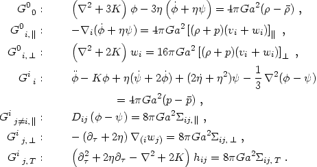(4.49) (4.50) (4.51) (4.52) (4.53) (4.54) (4.55)

As in the synchronous gauge, the scalar and vector modes satisfy initial-value (ADM) constraints (eqs. 4.49-4.51) in addition to evolution equations. However, it is remarkable that in the Poisson gauge we can obtain the scalar and vector potentials directly from the instantaneous stress-energy distribution with no time integration required. This is clear for - and w, both of which obey elliptic equations with no time derivatives (eqs. 4.53 and 4.51, respectively). By combining the ADM energy and longitudinal momentum constraint equations we can also get an instantaneous equation for :

(4.56)

Bardeen (1980) defined the matter perturbation variable _m ( + 3 _f / and noted that it is the natural measure of the energy density fluctuation in the normal (inertial) frame at rest with the matter such that v + w = 0 (recall the discussion in section 4.3). However, for our analysis we will remain in the comoving frame of the Poisson gauge, in which case / and not _m is the density fluctuation.

We can show that for nonrelativistic matter the field equations we have obtained reduce to the Newtonian forms. First, it is clear that in the non-cosmological limit ( = K = 0), eq. (4.56) reduces to the Poisson equation. For 0 the longitudinal momentum density _f is also a source for , but it is unimportant for perturbations with | / |>> v_Hv / c² where v_H is the Hubble velocity across the perturbation. Next, consider the implications of the fact that the shear stress for any physical system is at most O( c_s²) where c_s is the characteristic thermal speed of the gas particles. (For a collisional gas the shear stress is much less than this.) Equation (4.53) then implies that the relative difference between and is no more than O(c_s / c)². Third, eq. (4.51) implies that the vector potential w ~ (v_H / c)²v. Thus, the deviations from the Newtonian results are all O(v / c)². Poisson gauge gives the relativistic cosmological generalization of Newtonian gravity.

There are still more remarkable features of the Poisson gauge. First, the Poisson gauge metric perturbation variables are almost always small in the nonrelativistic limit (|| << c², v² << c²), in contrast with the synchronous gauge variables h_ij, which become large when | / |> 1. (However, Bardeen 1980 shows that the relative numerical merits of these two gauges can reverse for isocurvature perturbations of size larger than the Hubble distance.) Second, if (, , w, h) are very small, they - but not necessarily their derivatives! - may be neglected to a good approximation, in which case the Poisson gauge coordinates reduce precisely to the Eulerian coordinates used in Newtonian cosmology. Finally, it is amazing that the scalar and vector potentials depend solely on the instantaneous distribution of stress-energy - in fact, only the energy and momentum densities and the shear stress are required. Only the tensor mode - gravitational radiation - follows unambiguously from a time evolution equation. In fact, it obeys precisely the same equation as in the synchronous gauge (with a factor of 2 difference owing to our different definitions) because tensor perturbations are gauge-invariant - coordinate transformations involving 3-scalars and a 3-vector cannot change a 3-tensor (leaving aside the special case of eq. 4.17 for a closed space).

² The same gauge has been proposed recently by Bombelli, Couch & Torrence (1994), who call it "cosmological gauge." However, I prefer the name Poisson gauge because cosmology - i.e., nonzero - is irrelevant for the definition and physical interpretation of this gauge. Although I have seen no earlier discussion of Poisson gauge in the literature, its time slicing corresponds with the minimal shear hypersurface condition of Bardeen (1980). Back.