4.7. Physical content of the Einstein equations

In the last section we showed that the Poisson gauge variables (, , w) are given by the instantaneous distributions of energy density, momentum density, and shear stress (longitudinal momentum flux density). Is this action at a distance in general relativity?

We showed in eq. (4.47) that the Poisson gauge can be transformed to any other gauge. In the cosmological Lorentz gauge (see Misner et al. 1973 for the noncosmological version) all metric perturbation components obey wave equations. Therefore, the solutions in Poisson gauge must be causal despite appearances to the contrary.

There is a precedent for this type of behavior: the Coulomb gauge of electromagnetism. With ^. A = 0, eqs. (4.45) become

(4.57)

We have separated the current density into longitudinal and transverse parts. The similarity of the first two (scalar) equations to eqs. (4.49) and (4.50) is striking. The similarity would be even more striking if we were to use comoving coordinates rather than treating x and here as flat spacetime coordinates. As an exercise one can show that with comoving coordinates, and J will be multiplied by a² and that becomes + . The last step follows when one distinguishes time derivatives at fixed x from those at fixed ax.

Are we to conclude that electromagnetism also violates causality, because the electric potential depends only on the instantaneous Distribution of charge? No! To understand this let us examine the Coulomb and Ampère laws in flat spacetime for the fields rather than the potentials:

(4.58)

The Ampère law has been split into longitudinal and transverse parts. We see that the longitudinal electric field indeed is given instantaneously by the charge density. Because the photon is a massless vector particle, only the transverse part of the electric and magnetic fields is radiative, and its source is given by the transverse current density:

(4.59)

But how does this restore causality? To see how, let us consider the following example. Suppose that there is only one electric charge in the universe and initially it is at rest in the lab frame. If the charge moves - even much more slowly than the speed of light - E_|| - the solution to the Coulomb equation - is changed everywhere instantaneously. It must be therefore that E also changes instantaneously in such a way as to exactly cancel the acausal behavior of E_||.

This indeed happens, as follows. First, note that the motion of the charge generates a current density J = J_|| + J. The longitudinal and transverse parts separately extend over all space (and are in this sense acausal) while their sum vanishes away from the charge (as do ^. J_|| and × J). The magnetic and transverse electric fields obey eqs. (4.59). Because J is distributed over all space but × J is not, retarded-wave solutions for B are localized and causal while those for E are not. However, when E_|| is added to E, one finds that the net electric field is causal (Brill & Goodman 1967). It is a useful exercise to show this in detail.

Now that we understand how causality is maintained, what is the use of the longitudinal part of the Ampère law, - E_|| = 4 J_||? The answer is, to ensure charge conservation, which is implied by combining the time derivative of the Coulomb law with the divergence of the Ampère law:

(4.60)

Charge conservation is built into the Coulomb and Ampère laws. This remarkable behavior occurs because electromagnetism is a gauge theory. Gauge invariance effectively provides a redundant scalar field equation whose physical role is to enforce charge conservation. From Noether's theorem (e.g., Goldstein 1980), a continuous symmetry (in this case, electromagnetic gauge invariance) leads to a conserved current.

General relativity is also a gauge theory. Coordinate invariance - a continuous symmetry - leads to conservation of energy and momentum. As a result there are redundant scalar and vector equations [eqs. (4.50), (4.52), and (4.54)] whose role is to enforce the conservation laws [eqs. (4.24) and (4.25)]. We are free to use the action-at-a-distance field equations for the scalar and vector potentials in Poisson gauge because, when they are converted to fields and combined with the gravitational radiation field, the resulting behavior is entirely causal.

The analogy with electromagnetism becomes clearer if we replace the gravitational potentials by fields. We define the "gravitoelectric" and "gravitomagnetic" fields (Thorne, Price & Macdonald 1986; Jantzen, Carini & Bini 1992)

(4.61)

using the Poisson gauge variables and w. In section 4.8 we shall see how these fields lead to "forces" on particles similar to the Lorentz forces of electromagnetism. For now, however, we are interested in the fields themselves.

Note that g and H are invariant under the transformation - , w w + . In the noncosmological limit ( = 0) this is a gauge transformation corresponding to transformation of the time coordinate (cf. eqs. 4.39 and 4.40). However, gauge transformations in general relativity are complicated by the fact that they change the coordinates and fields as well as the potentials. For example, the terms in eq. (4.40) arise because the transformed metric is evaluated at the old coordinates. Thus, g should acquire a term under a true gauge (coordinate) transformation, which is incompatible with eq. (4.61). The actual transformation ( - , w w + ) is not a coordinate transformation. General relativity differs from electromagnetism in that gauge transformations change not just the potentials but also the coordinates used to evaluate the potentials; remember that the potentials define the perturbed coordinates! Only in a simple coordinate system, such as Poisson gauge - the gravitational analogue of Coulomb gauge - is it possible to see a simple relation between fields and potentials similar to that of electromagnetism.

In the limit of comoving distance scales small compared with the curvature distance |K|^-1/2 and the Hubble distance ^-1, and nonrelativistic shear stresses, the gravitoelectric and gravitomagnetic fields obey a gravitational analogue of the Maxwell equations:

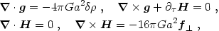(4.62)

where f = ( + p)(v + w) is the momentum density in the normal (inertial) frame. (You may derive these equations using eqs. 4.49, 4.50, 4.53, and 4.61.) These equations differ from their electromagnetic counterparts in three essential ways: (1) the sources have opposite sign (gravity is attractive), (2) the transverse momentum density has a coefficient 4 times larger than the transverse electric current (gravity is a tensor and not a vector theory), and (3) there is no "displacement current" - g in the transverse Ampère law for × H. Recalling that Maxwell added the electric displacement current precisely to conserve charge and thereby obtained radiative (electromagnetic wave) solutions, we understand the difference here: the vector component of gravity is nonradiative. Unlike the photon, the graviton is a spin-2 particle (or would be if we could quantize general relativity!), so radiative solutions appear only for the (transverse-traceless) tensor potential h_ij. In fact, the vector potential is nonradiative precisely because it is needed to ensure momentum conservation; mass conservation is already taken care of by the scalar potential. Recall the role of the ADM constraint equations discussed in section 4.4. Gravity has more conservation laws to maintain than electromagnetism and consequently needs more fields to constrain.

Obtaining this physical insight into general relativity is much easier in the Poisson gauge than in the synchronous gauge. This fact alone is a good reason for preferring the former. When combined with the other advantages (simpler equations, no time evolution required for the scalar and vector potentials, reduction to the Newtonian limit, no nontrivial gauge modes, and lack of unphysical coordinate singularities), the superiority of the Poisson gauge should be clear.

Although the physical picture we have developed for gravity in analogy with electromagnetism is beautiful, it is inexact. Not only have we linearized the metric, we have also neglected cosmological effects in eqs. (4.62). We shall see in section 4.9 how to obtain exact nonlinear equations for (the gradients of) the gravitational fields.